In our previous post, we discussed enhancing edges, sometimes known as “edge detection”, although as we said this is a slightly misleading term. In this post we will explore one of the more interesting image processing algorithms for finding the actual edge locations for lines, and their slopes.
The algorithm we will explore is the “Hough Transform”, and I am always amazed that someone (Paul Hough, for whom it is named) could come up with a method such as this one. In many books it is not thoroughly explained, so I will attempt to really pick it apart in order that you can really get the hang of it.
First, recall that a line can be represented by the formula y = mx + b; Ok, now forget that, because that formula doesn’t work when the line is vertical – the slope becomes infinite, and y becomes undefined – technically known as a singularity.
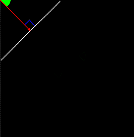
So, what’s another way to represent a line? Well I will just jump right to the way that the Hough Transform thinks about lines. There are three main parts to this way of representing lines – first, the point at the origin of the image (0,0). Second, a line of a certain distance (we’ll call this line r) that starts at the origin, and third, an angle we’ll call theta (?) which is the amount that r is rotated in order to be perpendicular to the line we are defining – i.e. the line we are looking for. So, a theoretically infinite line can be uniquely identified by the origin, r, and theta, and actually all we need are theta and r because the origin can be assumed to be the same throughout – (0,0).
So, as we can see in the figure below, we have our original white line (let’s pretend we don’t see it ) in our image that we’re trying to locate. If we knew where it was, we could describe it by the angle ?, and the line r.
So, we can now define lines two different ways – in a coordinate space based on x and y values, i.e. the Cartesian System, or we can define them by angle and distance from the origin. How does this help us, though? Well, what Mr. Hough came up with was an algortihm that is both sophisticated and “brute force”, if that’s possible.
What the algorithm does is walk through every pixel in the image, looking for a pixel that could be part of a line. In the case of our image above, that means any pixel that is not black. So, in our image we look through the first line and we find the white pixel at (0,60).
Now, recall that we don’t really know where the white line is – we’re looking for it. So, we start by creating lines that pass through this point and calculating the r value for each line.
We can start by looping from ? = 0 – 180 degrees. We know that the x (col) is 60, and the y (row) is 0.
So, let’s compute the length of that line with zero rotation = and we get r = 60.
60 = 60 cos(0) + 0sin(0)
So, the first potential line candidate, is perpendicular to our horizontal line at (60,0):
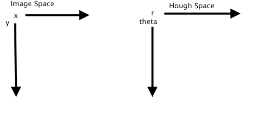
So, as we said we can represent lines by using an x, y coordinate system. We can also represent them by the angle theta and the line r. So, let’s make a new 2 dimension coordinate system, with one dimension theta and the other the length of r. Since we’re doing image processing, we can create an “image” to hold this data, with one dimension being theta and the other r. This type of image is know as the “Hough Space”. We are transforming points in the Cartesian space to information in the Hough Space. This information consists of “votes” for an angle and an r distance. Each “pixel” in the Hough Space will hold the sum of the votes for our candidate line based on theta, and r. Above we have our first line, so in the Hough Space we will add 1 vote for (theta, r) as (0, 60).
Hough Space (0,60,1) – angle 0, r 60, vote 1
Now, we continue this process for the next degree of theta, 1, and then 2, etc. Let’s move ahead to 10 degrees.
Now recall, we’re still on the first pixel that we found – the one at (60,0) – and this is the brute force part of the algorithm. For each degree, 0 – 180, we’re going to create a vote for every theta and r value in the Hough Space.
So, here we get a vote for (10, 59.085, 1).
So still staying at this first pixel location, we continue this process for each degree step. Since we already know our answer, let’s skip ahead to theta = 45 degrees:
Here we can see that the line is coincident with the line we’re looking for – and so we have our Hough Space vote at (45,42.42,1).
Now, we can see the pattern – as we “find” the white pixels in our line, we spin the blue line around and in this case it’s especially clear that each time that the blue line is coincident with the line we are looking for the votes will start to “add up” at that point – whereas the other positions of the blue line will generate smaller numbers of votes. Let’s try another white pixel at 45 degrees – let’s pick x = 48 and y = 12.
We calculate r as 48cos(45) + 12 sin(45)
and sure enough we get 42.42 so we have another vote for Hough Space (45,42.42) which means that the vote at that coordinate will increase by 1. And so in the Hough Space image at row 45 col 42.42 we will have 2 votes (assuming we really skipped ahead).
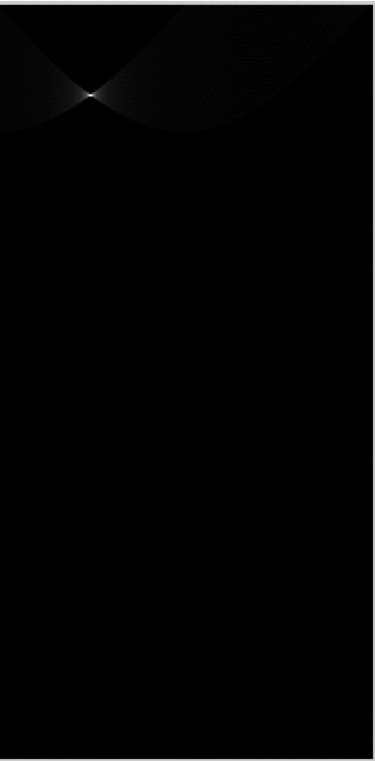
Now let’s run a version of the Hough Transform on our image, and see the resulting Hough Space image:
Here we see a small little blob, and the brightness of each pixel represents the number of votes for that r and theta. Let’s look at the underlying data in the image:
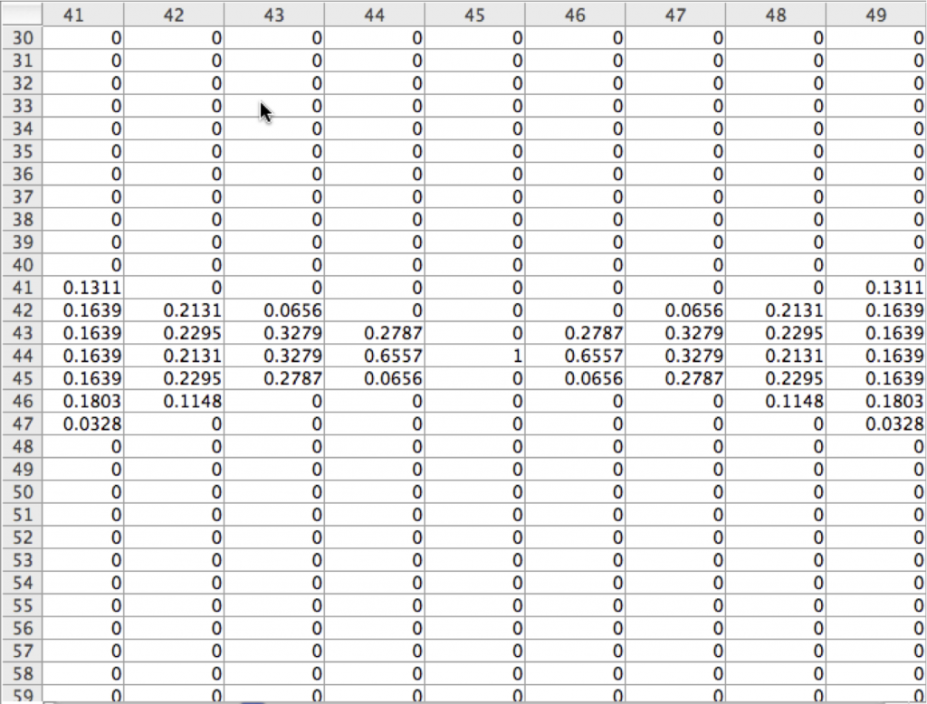
Here the columns represent the Angles, and the rows represent is the distance. The value in each entry is the number of votes, which is the brightness in the resulting Hough Space image.
The image data in the spreadsheet view above has been normalized to between 0 and 1.0, so, our “brightest” spot, a 1.0, is at 45 degrees! But wait – the distance r, as seen in the row numbers, is 44, and we had calculated 42.42. It turns out that there is a fair amount of inaccuracy in the Hough Transform, and special care needs to be taken to improve the accuracy. So, we are getting a very good result on the angle, but due to rounding and other types of errors, our r values are not quite exact. There are methods for improving these result – see the book mentioned at the end of this post for possible variations that can improve accuracy.
The final step of the Hough Transform is to walk through the image and find the maximum(s) and you will have your line or lines. How one does this depends more precisely what you are trying to accomplish. Perhaps you are looking for lines with specific angles, or perhaps at specific locations.
This covers the basics of the Hough Transform for locating lines. There are many variations on the Hough Transform – variations for finding circles, ellipses, and even general “shapes”. For more detail an excellent book is “Feature Extraction and Image Processing” by Mark S. Nixon and Alberto S Aguado.
Rick Frank
Dominion Software, Inc.
Hough Space Image of the Construction image in the first Edge Detection Post:
Matlab Code:
function [ houghImage ] = lineHough( image )
%create line hough transform image from input image
[rows cols] = size(image);
% our maximum is the euclidean distance across the image
radiusMax = round(sqrt(rows * rows +cols * cols));
% your threshold may vary.
thresh = max(max(image)) / 2;
%allocate our hough image space
houghImage = zeros(radiusMax,180);
for row = 1:rows
for col = 1:cols
% did we find a potential line pixel?
if image(row,col) > thresh
for theta = 1:180
r = round(col * cos(theta * pi/180.0) + row * sin(theta * pi/180));
if(r < radiusMax & r > 0)
houghImage(round(r),round(theta)) = houghImage(round(r),round(theta)) + 1;
end
end
end
end
end
% we have our image – scale it between 0.0 and 1.0 so that it
% is pleasing to the eye.
im = houghImage;
m = max(max(im));
im = im/m;
houghImage = im;
end


