
This is the third part of my series on my image processing work for GreenStand. If you haven’t read my previous posts, GreenStand is working to improve the environment and living conditions of places around the world by giving people incentives to plant trees. The trees absorb carbon, provide shade, and in the case of trees that bear fruits or nuts, create an ongoing economic benefit.
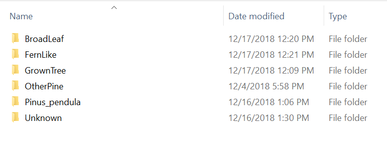
You may recall that the problem we’re trying to solve is to correctly identify a tree and its planter. To do this we are classifying the trees into categories – BroadLeaf, Pine (pinus_pendula), FernLike, GrownTree, and OtherPine. Additionally, we can use the Geo-spatial data that’s provided by the phone (its location in Latitude and Longitude).
I’ve also added a 5th category – “Unknown”, where I will put faces that are sometimes uploaded; the planters often have photos on their cell phones that are typically of themselves and those are included with the tree data.
Machine Learning
Machine Learning is a vast area of computer science, and is a subset of the more general topic of Artificial Intelligence. We’re going to experiment with just two basic algorithms from within the Machine Learning area; A Support Vector Machine, and a Convolutional Neural Network (Deep Learning).
Support Vector Machines
Support Vector Machines have been around since the 60’s, and have been heavily researched. Although the mathematics involved can be quite complex, the basic idea has an intuitive explanation.
Let’s imagine that you’re trying to classify 2 different objects. There are 40 objects all together and you plot their lengths and weights, which you obtained by measuring. You can then plot these objects, and you will notice that the data points tend to cluster around 2 points on the graph.

We can certainly see these 2 clusters pretty easily with our eyes. However, there’s an infinite number of lines we could draw between them, so what the best way to separate the clusters, especially in a different situation where the data clustering isn’t so obvious?
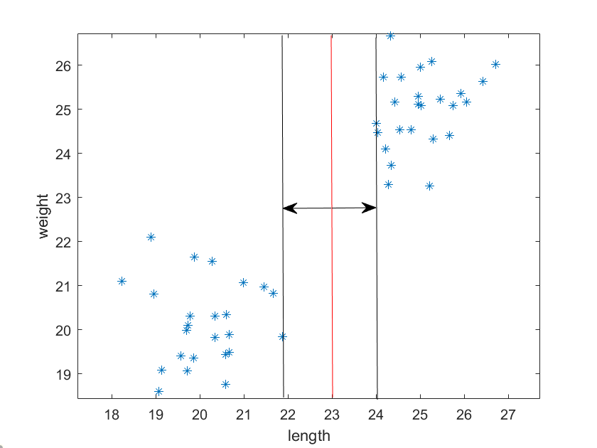
The vertical red line above shows one way to divide the two clusters, with the margins parallel to it.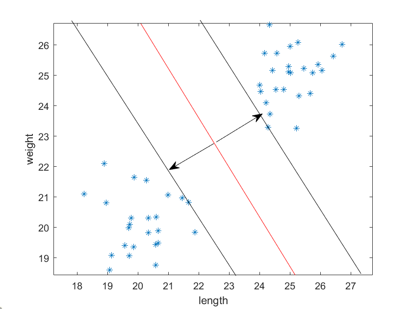
The vertical red line above shows another way to divide the two clusters; notice the margins lines parallel to it are further apart.
It turns out that the “best” way to divide the clusters is to find the line with the maximum margins between the edge of the clusters. Notice the two arrows perpendicular to the dividing line; these are the “support vectors”.
If we are in 3 dimensions, we want to find the plane that divides the clusters with the maximum margins. And in the general case of N dimensions, we want to find the hyper-plane that best divides the clusters in the same fashion. As mentioned, we have 6 classes, and it’s hard to visualize that many dimensions, but we can attempt to trust that such a space exists, and, our data may be linearly separable – separated by a 6 dimensional “line”.
We can see from the above that if we are trying to distinguish between many classes of data, the number of dimensions can get high and the calculations can become complex. Fortunately there are methods for multi-class partitioning that help simplify this problem. One way to reduce the dimensions is to use an ensemble of binary classifiers, and then a voting method to determine the likely outcome based on the whole ensemble’s decisions. In our Matlab implementation, we will use the function fitcecoc, whose name is an hint for the fact that it uses the “error-correcting output codes (ECOC) model” which reduces the problem of multi-class classification to a set of binary classifiers.
In [Dietterich,Bakiri,95], this ECOC method is described for classifying handwritten digits from 0-9. As an example description in their paper, six features are extracted for each digit. Here are the features and their abbreviations:
| Abbreviation | Meaning |
|---|---|
| vl | contains vertical line |
| hl | contains horizontal line |
| dl | contains diagonal line |
| cc | contains closed curve |
| ol | contains curve open to the left |
| or | contains curve open to the right |
The code words for the letters are in the table below:
| Class | vl | hl | dl | cc | ol | or |
|---|---|---|---|---|---|---|
| 0 | 0 | 0 | 0 | 1 | 0 | 0 |
| 1 | 1 | 0 | 0 | 0 | 0 | 0 |
| 2 | 0 | 1 | 1 | 0 | 1 | 0 |
| 3 | 0 | 0 | 0 | 0 | 1 | 0 |
| 4 | 1 | 1 | 0 | 0 | 0 | 0 |
| 5 | 1 | 1 | 0 | 0 | 1 | 0 |
| 6 | 0 | 0 | 1 | 1 | 0 | 1 |
| 7 | 0 | 0 | 1 | 0 | 0 | 0 |
| 8 | 0 | 0 | 0 | 1 | 0 | 0 |
| 9 | 0 | 0 | 1 | 1 | 0 | 0 |
In the simplest sense, when the software extracts the features, it computes what’s known as the Hamming Distance between the found bit pattern and the bit pattern in the coding table, which is simply the difference in the number of bits on in each pattern. The Hamming Distance between rows 4 and 5 above is simply one.
The distance between rows 4 and 5 turns out to be too small to be practical however; more bits must be added for the algorithm to be robust and truly error correcting. I won’t go into all the details here. One can refer to the original paper referenced below for more information on the implementations used in their testing.
Features for our clustering
To use this method for classifying our data, we need to extract some features from the images that can be used to create the kind of clusters of points we see above. As mentioned in the previous post, identifying objects of nature – as opposed to objects created by humans – can be more difficult since most of the research on finding objects in images centers around finding corners, straight lines, circles, etc. Objects that humans make, such as stop signs, car tires, lines in the road, etc.
One type of feature that has been used successfully to detect human figures in images is known as the Histogram of Oriented Gradients (HoG).
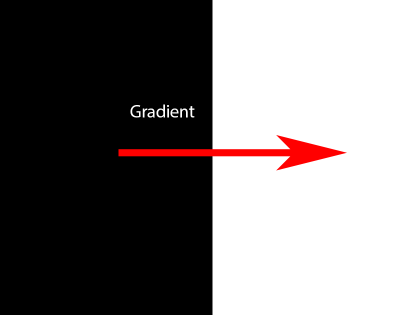
In the first image below, the arrow shows the gradient – the place in the image where the value of the pixels changes. In this case it goes from black (0) to white (255) so the gradient can be computed as the difference at that point (255 – 0 = 255).
The second image shows the gradient, but also the direction described as a counter-clockwise rotation.

By creating a histogram of the vectors over regions of the images – the magnitude of the gradient and the direction – one can create a feature descriptor of the shapes in each image. If similar shapes have similar directional gradient patterns, they can be used to as a set of features for that shape.
Matlab provide an easy to use interface to extract and display the HoG features:
[hog_NxN, plotNxN] = extractHOGFeatures(img,'CellSize', [8,8],'NumBins',18,'UseSignedOrientation',true);
figure;
imshow(img);
hold on;
% Visualize the HOG features

plot(plotNxN);

Let’s magnify a section to see more clearly what the gradients look like:

The commentary in the plot function describes exactly what we are seeing:
plot(visualization) plots the HOG features as an array of rose
% plots. Each rose plot shows the distribution of edge directions within a
% cell. The distribution is visualized by a set of directed lines whose
% lengths are scaled to indicate the contribution made by the gradients in
% that particular direction. The line directions are fixed to the bin
% centers of the orientation histograms and are between 0 and 360 degrees
% measured counterclockwise from the positive X axis. The bin centers are
% recorded in the BinCenters property.
%
Histogram of gradients features have been particularly good at detecting human pedestrian shapes. They have also been used to detect other types of objects with success. Will they work for our tree seedlings? We’ll have to try it out and see.
Preparing the data
In order to teach the computer what the images are, we need to first provide a set of “ground truth” images – images that a human recognizes as one type of plant or another – into a set of folders with each folder having the name we want to “label” each image in that folder. These we have to do by hand.
Matlab has a handy object type called an imageDataStore. When you create an imageDataStore, you pass in parameters that can make setting up your data flow simpler.
imds = imageDatastore(path,'IncludeSubfolders',true,'LabelSource','foldernames');
The Matlab function imageDataStore above is created from the path variable, which points to the parent path of our labeled folders, and takes the parameters “IncludeSubFolders” and “LabelSource”, which create an object that keeps track of the image locations by path name, and the Labels associated with each image
trainingFolder = 'C:\Users\rickf\Google Drive\Greenstand\SVM\Training';
imds = imageDatastore(trainingFolder,'IncludeSubfolders',true,'LabelSource','foldernames');
imdsAug = augmentedImageDatastore([300,300],imds,'OutputSizeMode','centercrop' );
Matlab also provides a nice helper object, the “augmentedImageDataStore”. This object can apply a number of image transforms – scaling, cropping, rotation, etc. – to your image when the image is read. This is very useful, as often the photos may be of different sizes, and the inputs to training algorithms – both for Machine Learning and Neural Networks – will almost always require the images to be all the same size. Here we are choosing to always center crop the images to 300 x 300 pixels.
dataTable = readByIndex(imdsAug,20);
img = dataTable{1,1}{1};
img = SegmentGreenWithOtsu(img);

[hog_NxN, plotNxN] = extHoGFeatures(img);
figure;
imshow(img);
hold on;
% Visualize the HOG features

plot(plotNxN);

hogFeatures = zeros(length(imds.Files),length(hog_NxN));
In the code above, we read in a random image to determine the size of the feature vectors so we can pre-allocate enough space to hold all the data ahead of time. We can also visualize the features to see that they make sense.
numImages = length(imds.Files);

for i = 1:numImages
    try
        path = imds.Files{i,1};
        dataTable = readByIndex(imdsAug,i);
        img = dataTable{1,1}{1};

       img = SegmentGreenWithOtsu(img);
        [features , ~] = extHoGFeatures(img);
        hogFeatures(i,:) = features;
    catch ME
        disp(ME);
    end
end
trainingLabels = imds.Labels;

save('trainingHoGData.mat','hogFeatures','trainingLabels','-v7.3');
Above, we loop through and grab the features for each image, and add them to our hogFeatures buffer. When we have finished all the images, we save the feature data and the labels to a .mat file to be read in later.
Training
Sit! Stay!
Whooo’s a good gurrrlll!
If you’ve ever trained a pet, you know you have to repeat the commands many times and offer a lot of rewards for correct behavior before the animal learns what you want them to do. It’s kind of similar when training a machine learning algorithm. We have to provide a lot of well labeled examples.
I’ve set up a set of testing folders with the layout like the training folders, but with different images. Let’s load in the training data we saved above and train and test our Support Vector Machine.
load trainingHoGData.mat;

classifier = fitcecoc(hogFeatures, trainingLabels);

testingFolder = 'C:\Users\rickf\Google Drive\Greenstand\SVM\Testing';
imds = imageDatastore(testingFolder,'IncludeSubfolders',true,'LabelSource','foldernames');
imdsAug = augmentedImageDatastore([300,300],imds,'OutputSizeMode','centercrop' );
Allocate the space for our test data
hogTestFeatures = zeros(length(imds.Files),length(hogFeatures));
Extract the testFeatures
for i = 1:length(imds.Files)
    try
        dataTable = readByIndex(imdsAug,i);
        img = dataTable{1,1}{1};
        img = SegmentGreenWithOtsu(img);

        [testFeatures , ~] = extHoGFeatures(img);
        hogTestFeatures(i,:) = testFeatures;
    catch ME
        disp(ME);
    end
end
Make class predictions using the test features.
predictedLabels = predict(classifier, hogTestFeatures);
testLabels = imds.Labels;
% Tabulate the results using a confusion matrix.
[confMat,order] = confusionmat(testLabels, predictedLabels);

figure
cm = confusionchart(confMat,order);

cm.ColumnSummary = 'column-normalized';
cm.RowSummary = 'row-normalized';
cm.Title = 'Plant Image Confusion Matrix';
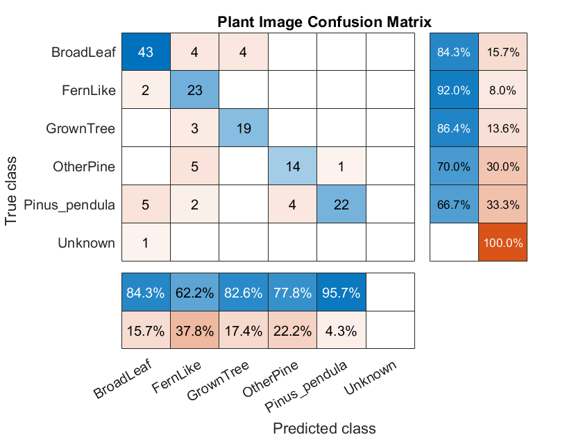
Matlab gives us a function to create a Confusion Matrix.
The matrix gives us a precise view of what the classifier got right, and what it got wrong. Here we can see we did pretty well, but there are a number of misclassified plants. Ideally we’d like to have the blue diagonal a darker shade. We can probably adjust parameters on our algorithm and data to improve the results.
But let’s move on to the latest advances in Machine Learning – Deep Learning with a Convolutional Neural Network – in the next post. We will see a significant improvement.
References
[Dietterich,Bakiri,95] Thomas G. Dietterich, G. B. (1995). Solving Multiclass Learning Problems via Error-Correcting Output Codes. Journal of Artificial Intelligence Research, 263-268.