I’ve recently been watching the online lectures of Dr. Joachim Hornegger’s Diagnostic Medical Imaging class. For anyone interested in state-of-the-art image processing techniques, especially related to medical imaging, these lectures are extremely useful and also have the side benefit of being entertaining (to geeks, at least).
A link to the course website is here.
What is Image Registration?
Let’s say that you have 2 pictures of the same object, or scene, taken at different times and also from different angles. If you want to see if anything has changed in the object or scene since the time the first picture was taken, it’s much easier if the pictures are lined up so that the object is not rotated, or moved up , down, left, or right. In the medical field, perhaps a tumor has changed over time and you want to align two pictures of the tumor in order to more clearly see any changes that might have taken place over time.
So we want to align the images, but we don’t know the angle or shift between the first and second pictures – and they might have used an x ray device for one image and an MRI for the other. and we must find a way to estimate this angle and/or shift as best as possible. We can then rotate or shift the picture so that the second picture appears to be in same position and angle as the first. Once this is done you can see the two pictures side by side and compare the object or scene without having to mentally rotate or shift the image.
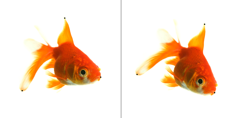
So, let’s look at some pictures. Here we have a picture of a goldfish, and then we have the same goldfish, but rotated by some number of degrees clockwise. How can we figure out what we need to do to get the second image to align back up with the first?
Point Correspondences
One way to make the image registration easier is to provide hints to the algorithm. A human can manually locate points in both images that are the “same” points in the two objects. You can see the black spots I placed on the fish images above. Once we have placed the corresponding points, we must then compute the transformation that takes us from picture 2 back to picture 1:
Note, the pictures above have selected points that look like they are in 3d, but in this example we just want to line up the fish in 2 dimensions. So we treat the spots as just 2d points, with an x coordinate and a y coordinate.
Imagine, a use for imaginary numbers!
You probably learned about imaginary, a.k.a complex, numbers in middle or high school, and at that time like most people I had very little idea of what use they might be. It just seemed to me to be one more kooky thing I had to remember for a test. It turns out, however, that there are actually many uses for them in practical applications. One of those uses is that they make finding the image registration parameters we need for our above problem relatively easy to obtain.
Professor Hornegger covers the details of the 2D-2D image transform using complex numbers quite thoroughly in the lecture and the lecture slides. I will go through the steps involved and also implement some Matlab code to perform the 2D – 2D Image Registration. What about 3D-3D, as mentioned in the title? Well we’ll get to that in part 2…
Complex numbers make things simple?
The useful thing about complex numbers for our situation is that they can be used for rotating points. Multiplying a complex number by another complex number results in a rotation and scaling of the first number by the second. If we create our complex number carefully, (by having it’s magnitude be 1.0) we can eliminate the scaling and just have the rotation.
Complex numbers have a “real” part and an “imaginary” part. We can plot these on a graph by having the x axis be for the “real part” and the y axis for the imaginary part of the complex number.
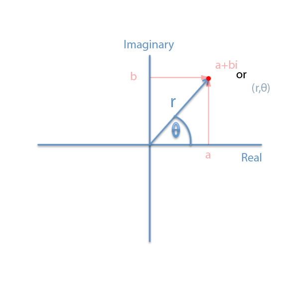
In the diagram above we see a red point that is described uniquely by two different coordinate representations. In the pink color, we see the complex number representation, and in the light blue color we see the polar representation, where the point can be uniquely described by the line length r and the rotation angle theta.
Diversion – deriving Euler’s Identity
Now we can set up some handy equivalencies, by noting the following:
a = r * cos(Θ)
b = r * sin(Θ)
So, we have
a + bi = r * cos(Θ) + r*i*sin(Θ) = r( cos(Θ) +i*sin(Θ))
For our purposes, we want to deal with only rotations, and no scaling. So, we limit our value of r to 1.0. This lets us take out the r, since it would be only a multiplication by 1.0.
a+bi = cos(Θ) + i*sin(Θ) or, if we create a new single letter for a + bi, let’s call it z, we can say
z = cos(Θ) + i*sin(Θ).
We can then take the derivative of this function of Θ, and we end up with
dz/d theta = -sin(Θ) + i*cos(Θ)
and then factoring out the i gives us
dz/d Θ = i(i*sin(Θ) + cos(Θ)).
This looks familiar – if we rearrange the right hand side we get
dz/d Θ = i(cos(Θ) + i*sin(Θ)), which is = i(z)!
So, dz/d Θ = i(z).
To solve this, let’s move the z’s to the same side, giving
dz/z = d Θ * i
Solving by integrating both sides give
ln(z) = Θ * i
exponentiating, that is making each side the exponent of the base e, gives
z = e ^ Θ*i
Now we have yet another way of representing complex numbers, using the constant e raised to the Θ i power.
This form is sometimes called the Euler form.
So what have we shown? Well, given the Euler representation of our complex number, of unit length, we can see that multiplying two complex numbers gives a rotation:
a = e^Θ[1] * i * e^Θ[2] * i = e^(Θ[1] + Θ[2])i as seen here:
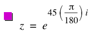
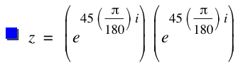
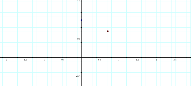
Above we see a complex point, represented by a unit length and 45 degree angle, multiplied by itself, giving a rotation of 45 degrees CCW. This demonstrates the idea that multiplying complex numbers provides us with an “easy” way to rotate points.
How does all this help us solve our problem with the fishes?
A rotation and translation of points can be described as below:

Here we see that we have a rotation matrix, R, that has Cos and Sin functions. To get the “best” answer, we want to minimize the sum of the squared differences between the rotatedPoint and the originalPoint rotated by Θ and translated by t. This give us the “best” answer, however the Cos and Sin functions make the problem non-linear, and that is not desired, because the solution will be difficult to compute.
By using the complex numbers this way we can set up a system of linear equations, which provides us a very straightforward way to solve for the unknown rotation and translation parameters.
We can set up this kind of equation with the complex numbers as follows:
C1 = unrotated complex point 1
C2 = unrotated complex point 2
C3 = unrotated complex point 3
C11 = rotated complex point 1
C22 = rotated complex point 2
C33 = rotated complex point 3
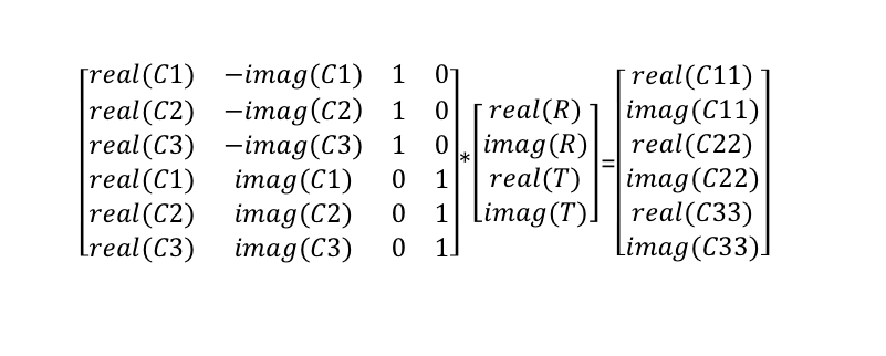
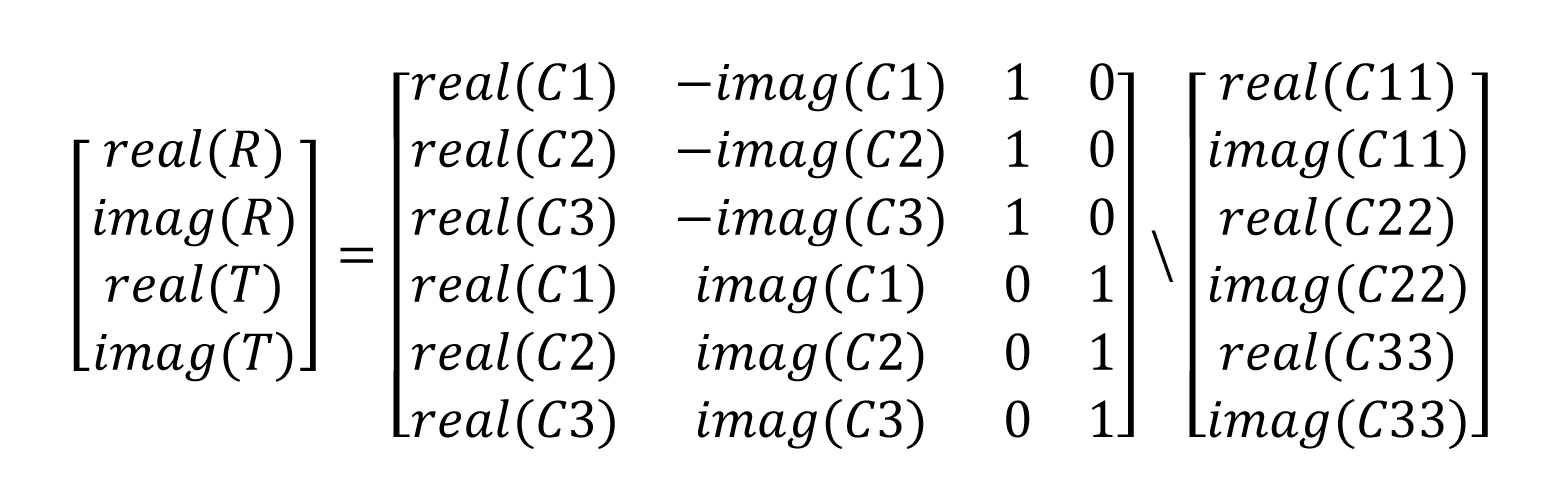
This matrix is the usual Ax = b system of linear equations. We can solved this for x in Matlab with the handy backslash operator, i.e. x = A\b.
Recall we are looking for the complex number R, which will be our rotation, and T which is our translation. These two complex numbers make up the vector x above.
So, we will have the following matrix to solve:
Let’s look at some code. Note, the matlab code below uses object oriented classes of my own design that wrap complex numbers, vectors, etc. However, the reader should be able to create similar classes to get the same results. I prefer the object oriented flavor of the code over the procedural flavor of matlab out of the box, so to speak.
%set up and read in the fishes...
clc;
clear all;
close all;
I1 = imread('Fish.png');
I2 = imread('Fish2.png');
subplot(1,2,1);
imshow(I1);
subplot(1,2,2);
imshow(I2);
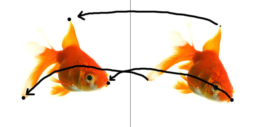
%the point correspondences - these are the human selected points.
p1 = [267,79];
p2 = [96,372];
p3 = [413,318];
p11 = [329,98];
p22 = [56,301];
p33 = [370,375];
[imR imC] = size(I1);
%NOTE, the image points are in "image coordinates, with (1,1) at top left.
% We flip these into cartesion form, with (0,0) in the bottom left.
p1 = imCoords2cartCoords(imR,p1);
p2 = imCoords2cartCoords(imR,p2);
p3 = imCoords2cartCoords(imR,p3);
p11 = imCoords2cartCoords(imR,p11);
p22 = imCoords2cartCoords(imR,p22);
p33 = imCoords2cartCoords(imR,p33);
% Create our objects, from real and imaginary axis points.
% these are the original points...
c1 = Complex(p1(1,1),p1(1,2));
c2 = Complex(p2(1,1),p2(1,2));
c3 = Complex(p3(1,1),p3(1,2));
% these are the rotated points...
c11 = Complex(p11(1,1),p11(1,2));
c22 = Complex(p22(1,1),p22(1,2));
c33 = Complex(p33(1,1),p33(1,2));
% create our custom object oriented plotting object...
plt = Plotting();
figure;
%draw the points....
plt.PlotComplex(c1,'O',[1 0 1],10,[1 0 1]);
hold on;
plt.PlotComplex(c2,'O',[1 1 0],10,[1 1 0]);
plt.PlotComplex(c3,'O',[0 1 1],10,[0 1 1]);
plt.PlotComplex(c11,'O',[1 0 0],10,[1 0 0]);
plt.PlotComplex(c22,'O',[0 1 0],10,[0 1 0]);
plt.PlotComplex(c33,'O',[0 0 1],10,[0 0 1]);
% Create the "A" matrix......
A = zeros(6,4);
A(1,1) = real(c1.c);
A(1,2) = -imag(c1.c);
A(2,1) = real(c2.c);
A(2,2) = -imag(c2.c);
A(3,1) = real(c3.c);
A(3,2) = -imag(c3.c);
A(1,3) = 1;
A(2,3) = 1;
A(3,3) = 1;
A(4,1) = imag(c1.c);
A(4,2) = real(c1.c);
A(5,1) = imag(c2.c);
A(5,2) = real(c2.c);
A(6,1) = imag(c3.c);
A(6,2) = real(c3.c);
A(4,4) = 1;
A(5,4) = 1;
A(6,4) = 1;
b = zeros(6,1);
% Set up the b matrix.....
b(1,1) = real(c11.c);
b(2,1) = real(c22.c);
b(3,1) = real(c33.c);
b(4,1) = imag(c11.c);
b(5,1) = imag(c22.c);
b(6,1) = imag(c33.c);
%SOLVE for X =
x = A\b
% the x vector now has r, and t...
r = Complex(x(1,1),x(2,1));
% just out of curiousity, display the angle, and the length of r
angleDegrees = r.angle() * 180/pi;
disp(angleDegrees);
disp(r.length());
% rotate our image....
I3 = imrotate(I2,angleDegrees,'bilinear','crop');
figure;
% and display it....
subplot(1,3,1);
imshow(I1);
subplot(1,3,2);
imshow(I2);
subplot(1,3,3);
imshow(I3);
So, the final result are seen below. The images are from left to right, the original, the rotated, and the registered image. Note that rotating the image creates a black background where the pixels are not in the original.
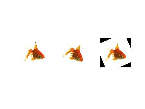
It turns out that the fish was rotated approximately 23 degrees…..
Next up in part 2……3d – 3d rotations with Quaternions….
Rick Frank