It’s not easy being green

This series of posts describes my image processing work for a non-profit organization called GreenStand. In case you didn’t read the first post, GreenStand’s mission is to give people in rural areas around the world incentives to plant trees, which can increase their standard of living and at the same time help the environment.

One of the tasks I’m working on is to help them identify the type of tree and the location of the tree, in order to correctly reimburse the planters. The planters, usually using a relatively inexpensive camera or phone, upload the images of the tree in order to be reimbursed. In the last post, I discussed and demonstrated an algorithm to detect when these photos were blurry, and out of focus. If the photo is out of focus, the planter can be asked by the GreenStand android app to take the photo again.

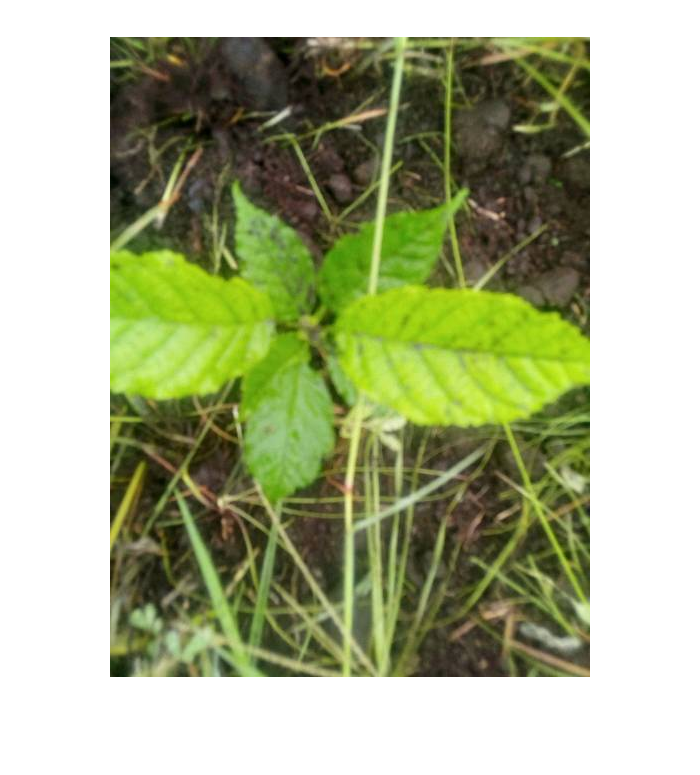
Now we begin the task of identifying the plants. The photo montage above shows four basic types of plants, and rather than try to identify individual species I will be classifying the images into 5 general categories: SmallPine (pinus pendula), BroadLeaf, OtherPine, GrownTree, and Fernlike.

For those people who might know something about deep learning, one might ask “Why not just modify AlexNet and use transfer learning on a Convolutional Neural Network”? Well, we’re going to be doing that later, but for now we can learn a lot about the data by first trying some other approaches.

In the table below, we can see two examples of the 5 categories we will try to classify:

 

		Pine (pinus pendula)
		Fernlike
		BroadLeaf
		OtherPine
		GrownTree

How can we approach identifying which category these plants belong to? What features in the images might we detect to help us? It’s a difficult problem, not only because of the “noise” – other green items in the photos – but because the corners, angles, and lines found in photos containing human made objects –  typical features used in computer vision, etc. –  are not that common in these images.

Can we first threshold the pictures to isolate the green objects from the other background “noise”?

The first thing one notices is the different shades for green. How would one go about thresholding – masking out the “green” areas – with that much variation in the color?

CIE L*a*b* color space

Since most of my image processing work is done in the colorless world of grayscale images – typical of medical and scientific imaging – I have not had to make use of color space processing very often. Fortunately, a lot of effort has been put into mapping colors into various forms of numeric values by others, and it looks like the L*a*b* space has what we need.

Notice in the view of the color space visualization below (courtesy Wikipedia), the red and green areas are at right angles to the blue and yellow.  Looking straight into the picture is decreasing lightness.

This means that we can isolate green hues more easily in this color space than in other spaces, since although green is composed of yellow and blue, in this model it is in a separate part of the space.

By Holger Everding – Own work, CC BY-SA 4.0,

Matlab has a unique “app” for doing color thresholding. The app (or a plugin, as I might call it) allows the developer to visually test parameters for doing color thresholding in 4 different color spaces.

We can choose the color space we want to edit in.

In the above tool, we can edit the L* (lightness), the a* channel (that’s the red to green) or the b* channel (that’s blue to yellow). If we move the slider in the a* channel we can isolate the green hues. We can also draw a polygon around the point cloud to further refine the color selection:

One thing to notice  – the histogram for a* is bi-modal. There are 2 distinct peaks. We can use this to our advantage.

 

Let’s see how well this works on an image with a plant with a different shade of green.

 

This works pretty well; I positioned the right hand slider on the a* channel between the 2 peaks.

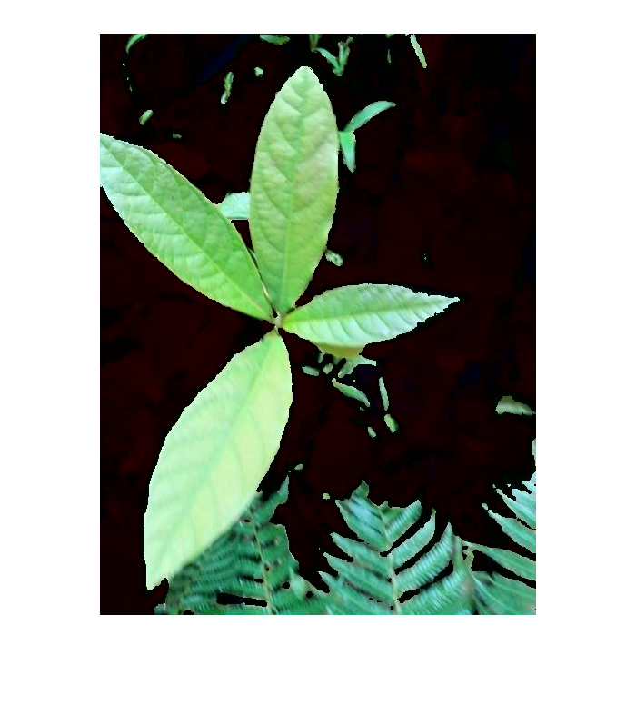
Here’s an idea – Otsu’s threshold works by finding the valley between 2 peaks as the place to “break” a grayscale image into foreground and background. If we apply Otsu’s method to the a* channel in L*a*b* space, many of our images can have the green segmentation done with the least error.

Let’s give it a try on these two images.

Load the image and normalize to 0…1

imshow(im1);

labIm1 = rgb2lab(im1);

channelA = labIm1(:,:,2);
mn = min(min(channelA))

channelA = channelA + abs(mn);
channelA = channelA./ max(max(channelA));

 

Perform Otsu Threshold on a* channel, set the L channel (brightness) to zero
to show only the pixels we want.

[counts, ~] = imhist(channelA);

cut = otsuthresh(counts)
channelL = labIm1(:,:,1);

channelL(channelA > cut) = 0;
labIm1(:,:,1) = channelL;
rgbImage = lab2rgb(labIm1);

imshow(rgbImage);

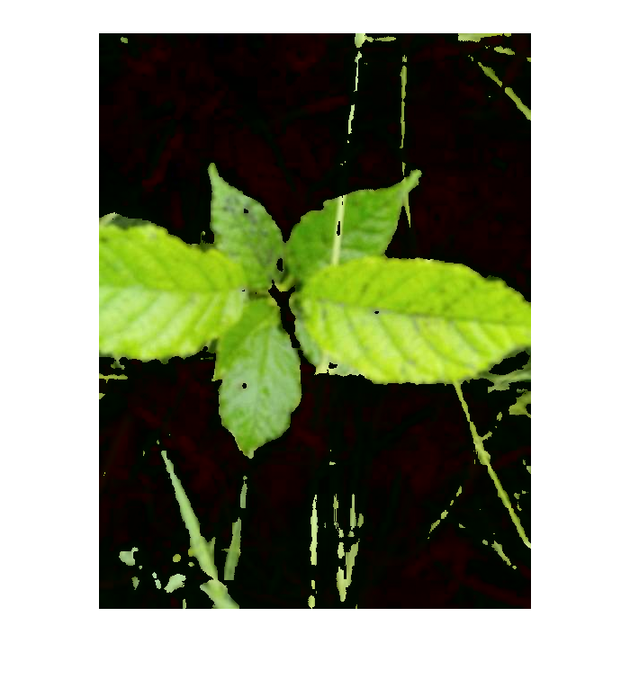
Seems to work pretty well. Let’s try the next image with the same code: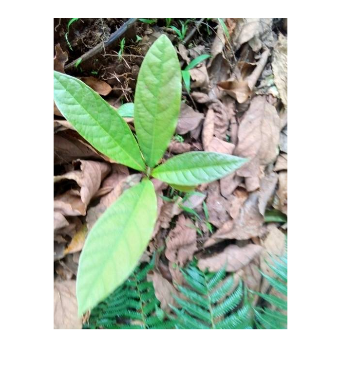

Up Next – extracting features from the segmented images.