Recently I’ve been working on a proof of concept  project for a client that uses Microsoft’s Mixed Reality Hololens device.

The Hololens is an intriguing device, giving the user – (or should I say “wearer” ?) – of the device the ability to place holograms – 3D “imaginary” shapes –  into the space they see in front of them. This is the “mixed” in Mixed Reality. You see through the clear lenses, and in addition, you see holographic objects in your view as if they were placed in the 3D space around you.

Relativity

Einstein showed us that there is no fixed point in space. Everything is relative. So, when you want to put a hologram in space, where is it exactly?

Similarly to DICOM images, where everything is relative to the patient, we can say with the hololens that everything is relative to the user. More precisely, relative to the sensors on the headset, but with calibration and reasonable care the origin point is roughly at the xz plane of the user’s eyes, with the y axis pointing up and the z axis pointing towards the user’s back.

Above, we see the wearer “gazing” at the fish hologram.

So, where exactly is the fish hologram?

Example Code

Microsoft provides a fair amount of Direct X example code on GitHub.
Let’s take a look at a simple example.

In the BasicHologram example, we see in BasicHologramMain.cpp at line 579

// The simplest way to render world-locked holograms is to create a stationary reference frame
// based on a SpatialLocator. This is roughly analogous to creating a "world" coordinate system
// with the origin placed at the device's position as the app is launched.
m_stationaryReferenceFrame = m_spatialLocator->CreateStationaryFrameOfReferenceAtCurrentLocation();


OK this makes sense. When you start up your application, when you want to grab a fixed, i.e. “world locked” frame, you use CreateStationaryFrameOfReferenceAtCurrentLocation().
If you position a hologram in this frame of reference, it will stay there, and if you move around it will stay in that position:

So above we see our intrepid goggle wearer moving, and the fish hologram stays positioned relative to the original frame of reference.

After working with this sample code for a bit, I then moved on to the next feature I needed; namely, access to the front facing color video camera.

You can’t get there from here

Alas, there just seemed to be no way to access the video stream from within this example code. Something to do with it being in the WinRT architecture vs the UWP architecture I think. But I gave up trying to figure it out, and moved to a code example that had access to the video camera, the HolographicFaceTracking example.

It didn’t take long to move my existing code over to this new example, and although it was in Microsoft’s proprietary Managed C++, I decided to bite the bullet and stick with this as a basis for my experimentation.

Everything seemed to be working correctly, and I was able to get the video stream and draw it to a texture so I could see it within the Hololens view. But after a while, I realized there was one problem. My Holographic shape was not behaving naturally;  as I moved towards it or away from it, it stayed the same size. Normally, if you viewed our friendly fish, positioned in the “world” coordinate system, it would get bigger as you walked towards it, as below:

Fish at one distance

Fish some steps closer.

 

However this wasn’t happening. It was puzzling. Until I finally realized that the FaceTracking Example just couldn’t be doing what it was saying it does.

The code in the BasicHologram example has the following comment when it places the hologram:

 // The simplest way to render world-locked holograms is to create a stationary reference frame
  // based on a SpatialLocator. This is roughly analogous to creating a "world" coordinate system
  // with the origin placed at the device's position as the app is launched.

Ok, that looks correct.

And the FaceTracking example has the same comment in the same area of code:

 // The simplest way to render world-locked holograms is to create a stationary reference frame
 // based on a SpatialLocator. This is roughly analogous to creating a "world" coordinate system
 // with the origin placed at the device's position as the app is launched.

I’m guessing that many of you have already guessed the problem; the code doesn’t match the comment.

In the BasicHologram example, we have the code that matches the comment.

m_stationaryReferenceFrame = m_spatialLocator->CreateStationaryFrameOfReferenceAtCurrentLocation();

And of course in the FaceTracking example, we have the code that doesn’t match the comment.

 m_referenceFrame = m_locator->CreateAttachedFrameOfReferenceAtCurrentHeading();

So, of course in the latter case, the hologram stays “fixed” but always relative to the origin of the user. It stays fixed only with respect to rotation, though. It moves with the user with respect to distance.

Above we see our fish gazer looking normally at the hologram.

If he takes a few steps backwards, with the “Attached Frame of Reference”, the fish moves with him, and so appears to not change size. But now the part that confused me.

If the user moves backwards, and then rotates their position, the hologram stays in place. So it’s invariant to rotation.

This all makes good sense to me now. And I’m moving forward on my experiment. But the moral of the story is: Trust comments, but verify.

Image Recognition with the Matlab Deep Learning Toolbox

After some time in the Artificial Intelligence Doghouse, Neural Networks regained status after Alex Krizhevsky, Ilya Sustkever, and Goeffrey Hinton won the Large Scale Visual Recognition Challenge in 2012 using their Neural Network, now known as AlexNet.

Details can be found in their paper.

The Matlab Deep Learning Toolbox makes it really easy to develop our own Deep Learning network to use for our tree seedling classification task. And, as it turns out, we can take advantage of the work done by the winners above by using their trained network to bootstrap our own network using a technique called Transfer Learning.

Overview of Deep Learning Neural Networks

A Neural Network is designed to mimic the way a biological neuron “Activates” on a given stimulus. How close it comes to recreating an actual biological neuron I will leave to the Neuroscientists to decide. But that is the concept. These neurons are then connected into “Layers”. The “Deep” part of “Deep Learning” refers to the fact that there are many layers of neurons in a particular network, therefore creating a “Deep” Neural Network.

Let’s take a look at the typical diagram for a section of a Neural Network:

The circles on the left are the activations. The lines connecting to the circle on the right are the weights. The circle on the right is the output which is the weighted sum of the activations plus a bias, b, plugged in as a parameter to σ(), which is a function known as a Rectifier which simply sets everything < 0 to 0. We’ll skip over the bias and the sigma function, as they are important but not essential to the basic concept.

These diagrams certainly didn’t mean all that much to me at first; as a programmer, I immediately thought “what does this look like in code”?

Well, it turns out that if you know a bit about image processing filters, it is easy to understand the basic concepts of convolutional neural networks.

It turns out that for the image specific tasks, like classifying photos, the activations are the input pixels. The weights are the values in an image filter. So, for instance, a filter could be a 3 by 3 edge detection filter,

-1	0	1
-1	0	1
-1	0	1

or any other type of image filter. The activations are the pixels of the input image, and so one is left with the “classic” image processing task of sliding a filter across an image, taking the dot product and setting a new pixel – potentially a new activation in the next layer.

Now, here’s where the “Learning” part of Deep Learning comes in. Instead of first specifying what filters to use, we tell the network what result we want, and it keeps adjusting the filters until it gets that result, or close to it. This feedback is known as back-propagation. So, let’s say we want to train the network to recognize an image with the label “Cat”. We keep feeding the images we want to be recognized as a Cat, and the algorithm keeps updating the filters until they agree that the images can be classified as a Cat. This is a bit of a simplification, but it is the basic essence of what is happening during the training process.

Once the network is trained properly, the filters will then be able to process an unseen before image as a “Cat”. 

With Matlab, we can actually look at the filters in the first layer of AlexNet.

Load AlexNet

net = alexnet;

Let’s look at the Layers:

net.Layers

ans = 
  25x1 Layer array with layers:

     1   'data'     Image Input                   227x227x3 images with 'zerocenter' normalization
     2   'conv1'    Convolution                   96 11x11x3 convolutions with stride [4  4] and padding [0  0  0  0]
     3   'relu1'    ReLU                          ReLU
     4   'norm1'    Cross Channel Normalization   cross channel normalization with 5 channels per element
     5   'pool1'    Max Pooling                   3x3 max pooling with stride [2  2] and padding [0  0  0  0]
     6   'conv2'    Convolution                   256 5x5x48 convolutions with stride [1  1] and padding [2  2  2  2]
     7   'relu2'    ReLU                          ReLU
     8   'norm2'    Cross Channel Normalization   cross channel normalization with 5 channels per element
     9   'pool2'    Max Pooling                   3x3 max pooling with stride [2  2] and padding [0  0  0  0]
    10   'conv3'    Convolution                   384 3x3x256 convolutions with stride [1  1] and padding [1  1  1  1]
    11   'relu3'    ReLU                          ReLU
    12   'conv4'    Convolution                   384 3x3x192 convolutions with stride [1  1] and padding [1  1  1  1]
    13   'relu4'    ReLU                          ReLU
    14   'conv5'    Convolution                   256 3x3x192 convolutions with stride [1  1] and padding [1  1  1  1]
    15   'relu5'    ReLU                          ReLU
    16   'pool5'    Max Pooling                   3x3 max pooling with stride [2  2] and padding [0  0  0  0]
    17   'fc6'      Fully Connected               4096 fully connected layer
    18   'relu6'    ReLU                          ReLU
    19   'drop6'    Dropout                       50% dropout
    20   'fc7'      Fully Connected               4096 fully connected layer
    21   'relu7'    ReLU                          ReLU
    22   'drop7'    Dropout                       50% dropout
    23   'fc8'      Fully Connected               1000 fully connected layer
    24   'prob'     Softmax                       softmax
    25   'output'   Classification Output         crossentropyex with 'tench' and 999 other classes

We can take a look at the 2nd layer and visualize the image filters. There are 96 filters, 11 pixels by 11 pixels by 3 pixels (one set of pixels each for R, G, B colors).

We offset the pixels all into the positive range so we can see them more easily, then write them as a tiff file.

layer = net.Layers(2);
img = imtile(layer.Weights);
mn = min(min(min(img)));
img = img - mn;

imgu = uint8(img.*255);

imwrite(imgu,'Tiles.tif','tif');

This is pretty interesting. 96 image filters that were “learned” from the 1.2 million images with 1000 different labels. I also notice the cyan and green colors, which remind me of the Lab color space from a previous post.

There a lot of details that one can go into here, of course. We’ll skip ahead to how we can use this network to recognize our own images.

Transfer Learning

It turns out that we can retrain an existing network to classify our seedlings using what is known as “Transfer Learning”. Using the Matlab Deep Learning Toolbox, we can do this by replacing two of the layers in the original AlexNet with our own.

First, we load the network, and set up a path to our Labeled image folders.

net = alexnet;
imagePath = 'C:\Users\rickf\Google Drive\Greenstand\TestingAndTraining';

 

We can set up our datastore, and use a Matlab helper function to pick 80 percent of the images for training. In addition, the augmentedImageDatastore() function let’s us scale the images to the required 227×227 inputs that AlexNet requires.

imds = imageDatastore(imagePath,'IncludeSubfolders',true,'LabelSource','foldernames');
[trainIm, testIm] = splitEachLabel(imds, 0.8,'randomized')

trainData = augmentedImageDatastore([227 227], trainIm)
testData = augmentedImageDatastore([227 227], testIm)

If we look above we can see that the final layers in the AlexNet network are set up for 1000 different labels.

23 'fc8' Fully Connected 1000 fully connected layer 
24 'prob' Softmax softmax 
25 'output' Classification Output crossentropyex with 'tench' and 999 other classes

What we need to do is to replace layer 23 with a fully connected 6 input layer (for our 6 labels),
and replace 25 with a new classifier that will accept those 6 inputs from the softmax layer.

layer(23) = fullyConnectedLayer(6,'Name','fcfinal');
layer(end) = classificationLayer('Name','treeClassification');

opts = trainingOptions('adam','InitialLearnRate',0.0001,'Plots','training-progress','MaxEpochs',10);
[net,info] = trainNetwork(trainData,layer,opts);

We specified the option to plot progress, which is shown above.

The final results can be seen in our confusion matrix.

Much better results that the Support Vector Machine, and no color segmentation was needed!

I  would suspect with more training data we can get the Broadleaf and Fernlike classifications to improve. We’ll try that, and then put the network to a test of classifying unseen new images in the next post.

 

This is the third part of my series on my image processing work for GreenStand. If you haven’t read my previous posts, GreenStand is working to improve the environment and living conditions of places around the world by giving people incentives to plant trees. The trees absorb carbon, provide shade, and in the case of trees that bear fruits or nuts, create an ongoing economic benefit.

You may recall that the problem we’re trying to solve is to correctly identify a tree and its planter. To do this we are classifying the trees into categories – BroadLeaf, Pine (pinus_pendula), FernLike, GrownTree, and OtherPine. Additionally, we can use the Geo-spatial data that’s provided by the phone (its location in Latitude and Longitude).

I’ve also added a 5th category – “Unknown”, where I will put faces that are sometimes uploaded; the planters often have photos on their cell phones that are typically of themselves and those are included with the tree data.

Machine Learning

Machine Learning is a vast area of computer science, and is a subset of the more general topic of Artificial Intelligence. We’re going to experiment with just two basic algorithms from within the Machine Learning area; A Support Vector Machine, and a Convolutional Neural Network (Deep Learning).

Support Vector Machines

Support Vector Machines have been around since the 60’s, and have been heavily researched. Although the mathematics involved can be quite complex, the basic idea has an intuitive explanation.

Let’s imagine that you’re trying to classify 2 different objects. There are 40 objects all together and you plot their lengths and weights, which you obtained by measuring. You can then plot these objects, and you will notice that the data points tend to cluster around 2 points on the graph.

We can certainly see these 2 clusters pretty easily with our eyes.  However, there’s an infinite number of lines we could draw between them, so what the best way to separate the clusters, especially in a different situation where the data clustering isn’t so obvious?

The vertical red line above shows one way to divide the two clusters, with the margins parallel to it.

The vertical red line above shows another way to divide the two clusters; notice the margins lines parallel to it are further apart.

It turns out that the “best” way to divide the clusters is to find the line with the maximum margins between the edge of the clusters. Notice the two arrows perpendicular to the dividing line; these are the “support vectors”.

If we are in 3 dimensions, we want to find the plane that divides the clusters with the maximum margins. And in the general case of N dimensions, we want to find the hyper-plane that best divides the clusters in the same fashion. As mentioned, we have 6 classes, and it’s hard to visualize that many dimensions, but we can attempt to trust that such a space exists, and, our data may be linearly separable – separated by a 6 dimensional “line”.

We can see from the above that if we are trying to distinguish between many classes of data, the number of dimensions can get high and the calculations can become complex.  Fortunately there are methods for multi-class partitioning that help simplify this problem. One way to reduce the dimensions is to use an ensemble of binary classifiers, and then a voting method to determine the likely outcome based on the whole ensemble’s decisions. In our Matlab implementation, we will use the function fitcecoc, whose name is an hint for the fact that it uses the “error-correcting output codes (ECOC) model” which reduces the problem of multi-class classification to a set of binary classifiers.

In [Dietterich,Bakiri,95], this ECOC method is described for classifying handwritten digits from 0-9. As an example description in their paper, six features are extracted for each digit. Here are the features and their abbreviations:

Abbreviation	Meaning
vl	contains vertical line
hl	contains horizontal line
dl	contains diagonal line
cc	contains closed curve
ol	contains curve open to the left
or	contains curve open to the right

The code words for the letters are in the table below:

Class	vl	hl	dl	cc	ol	or
0	0	0	0	1	0	0
1	1	0	0	0	0	0
2	0	1	1	0	1	0
3	0	0	0	0	1	0
4	1	1	0	0	0	0
5	1	1	0	0	1	0
6	0	0	1	1	0	1
7	0	0	1	0	0	0
8	0	0	0	1	0	0
9	0	0	1	1	0	0

In the simplest sense, when the software extracts the features, it computes what’s known as the Hamming Distance between the found bit pattern and the bit pattern in the coding table, which is simply the difference in the number of bits on in each pattern. The Hamming Distance between rows 4 and 5 above is simply one.

The distance between rows 4 and 5 turns out to be too small to be practical however; more bits must be added for the algorithm to be robust and truly error correcting. I won’t go into all the details here. One can refer to the original paper referenced below for more information on the implementations used in their testing.

Features for our clustering

To use this method for classifying our data, we need to extract some features from the images that can be used to create the kind of clusters of points we see above. As mentioned in the previous post, identifying objects of nature – as opposed to objects created by humans – can be  more difficult since most of the research on finding objects in images centers around finding corners, straight lines, circles, etc. Objects that humans make, such as stop signs, car tires, lines in the road, etc.

One type of feature that has been used successfully to detect human figures in images is known as the Histogram of Oriented Gradients (HoG).

In the first image below, the arrow shows the gradient – the place in the image where the value of the pixels changes. In this case it goes from black (0) to white (255) so the gradient can be computed as the difference at that point (255 – 0 = 255).

The second image shows the gradient, but also the direction described as a counter-clockwise rotation.

By creating a histogram of the vectors over regions of the images – the magnitude of the gradient and the direction – one can create a feature descriptor of the shapes in each image. If similar shapes have similar directional gradient patterns, they can be used to as a set of features for that shape.

Matlab provide an easy to use interface to extract and display the HoG features:

[hog_NxN, plotNxN] = extractHOGFeatures(img,'CellSize', [8,8],'NumBins',18,'UseSignedOrientation',true);
figure;
imshow(img);
hold on;
% Visualize the HOG features

plot(plotNxN);

Let’s magnify a section to see more clearly what the gradients look like:

The commentary in the plot function describes exactly what we are seeing:

plot(visualization) plots the HOG features as an array of rose
% plots. Each rose plot shows the distribution of edge directions within a
% cell. The distribution is visualized by a set of directed lines whose
% lengths are scaled to indicate the contribution made by the gradients in
% that particular direction. The line directions are fixed to the bin
% centers of the orientation histograms and are between 0 and 360 degrees
% measured counterclockwise from the positive X axis. The bin centers are
% recorded in the BinCenters property.
%

Histogram of gradients features have been particularly good at detecting human pedestrian shapes. They have also been used to detect other types of objects with success. Will they work for our tree seedlings? We’ll have to try it out and see.

Preparing the data

In order to teach the computer what the images are, we need to first provide a set of “ground truth” images – images that a human recognizes as one type of plant or another – into a set of folders with each folder having the name we want to “label” each image in that folder. These we have to do by hand.

Matlab has a handy object type called an imageDataStore. When you create an imageDataStore, you pass in parameters that can make setting up your data flow simpler.

imds = imageDatastore(path,'IncludeSubfolders',true,'LabelSource','foldernames');

The Matlab function imageDataStore above is created from the path variable, which points to the parent path of our labeled folders, and takes the parameters “IncludeSubFolders” and “LabelSource”, which create an object that keeps track of the image locations by path name, and the Labels associated with each image

trainingFolder = 'C:\Users\rickf\Google Drive\Greenstand\SVM\Training';
imds = imageDatastore(trainingFolder,'IncludeSubfolders',true,'LabelSource','foldernames');
imdsAug = augmentedImageDatastore([300,300],imds,'OutputSizeMode','centercrop' );

Matlab also provides a nice helper object, the “augmentedImageDataStore”. This object can apply a number of image transforms – scaling, cropping, rotation, etc. – to your image when the image is read. This is very useful, as often the photos may be of different sizes, and the inputs to training algorithms –  both for Machine Learning and Neural Networks –  will  almost always require the images to be all the same size. Here we are choosing to always center crop the images to 300 x 300 pixels.

dataTable = readByIndex(imdsAug,20);
img = dataTable{1,1}{1};
img = SegmentGreenWithOtsu(img);

[hog_NxN, plotNxN] = extHoGFeatures(img);
figure;
imshow(img);
hold on;
% Visualize the HOG features

plot(plotNxN);

hogFeatures = zeros(length(imds.Files),length(hog_NxN));

In the code above, we read in a random image to determine the size of the feature vectors so we can pre-allocate enough space to hold all the data ahead of time. We can also visualize the features to see that they make sense.

numImages = length(imds.Files);

for i = 1:numImages
    try
        path = imds.Files{i,1};
        dataTable = readByIndex(imdsAug,i);
        img = dataTable{1,1}{1};

       img = SegmentGreenWithOtsu(img);
        [features , ~] = extHoGFeatures(img);
        hogFeatures(i,:) = features;
    catch ME
        disp(ME);
    end
end
trainingLabels = imds.Labels;

save('trainingHoGData.mat','hogFeatures','trainingLabels','-v7.3');

Above, we loop through and grab the features for each image, and add them to our hogFeatures buffer. When we have finished all the images, we save the feature data and the labels to a .mat file to be read in later.

Training

Sit! Stay!
Whooo’s a good gurrrlll!

 

If you’ve ever trained a pet, you know you have to repeat the commands many times and offer a lot of rewards for correct behavior before the animal learns what you want them to do. It’s kind of similar when training a machine learning algorithm. We have to provide a lot of well labeled examples.

I’ve set up a set of testing folders with the layout like the training folders, but with different images. Let’s load in the training data we saved above and train and test our Support Vector Machine.

load trainingHoGData.mat;

classifier = fitcecoc(hogFeatures, trainingLabels);

testingFolder = 'C:\Users\rickf\Google Drive\Greenstand\SVM\Testing';
imds = imageDatastore(testingFolder,'IncludeSubfolders',true,'LabelSource','foldernames');
imdsAug = augmentedImageDatastore([300,300],imds,'OutputSizeMode','centercrop' );

Allocate the space for our test data

hogTestFeatures = zeros(length(imds.Files),length(hogFeatures));

Extract the testFeatures

for i = 1:length(imds.Files)
    try
        dataTable = readByIndex(imdsAug,i);
        img = dataTable{1,1}{1};
        img = SegmentGreenWithOtsu(img);

        [testFeatures , ~] = extHoGFeatures(img);
        hogTestFeatures(i,:) = testFeatures;
    catch ME
        disp(ME);
    end
end

Make class predictions using the test features.
predictedLabels = predict(classifier, hogTestFeatures);
testLabels = imds.Labels;
% Tabulate the results using a confusion matrix.
[confMat,order] = confusionmat(testLabels, predictedLabels);

figure
cm = confusionchart(confMat,order);

cm.ColumnSummary = 'column-normalized';
cm.RowSummary = 'row-normalized';
cm.Title = 'Plant Image Confusion Matrix';

Matlab gives us a function to create a Confusion Matrix.

The matrix gives us a precise view of what the classifier got right, and what it got wrong. Here we can see we did pretty well, but there are a number of misclassified plants. Ideally we’d like to have the blue diagonal a darker shade. We can probably adjust parameters on our algorithm and data to improve the results.

But let’s move on to the latest advances in Machine Learning – Deep Learning with a Convolutional Neural Network – in the next post. We will see a significant improvement.

 

References

[Dietterich,Bakiri,95] Thomas G. Dietterich, G. B. (1995). Solving Multiclass Learning Problems via Error-Correcting Output Codes. Journal of Artificial Intelligence Research, 263-268.

 

 

It’s not easy being green

This series of posts describes my image processing work for a non-profit organization called GreenStand. In case you didn’t read the first post, GreenStand’s mission is to give people in rural areas around the world incentives to plant trees, which can increase their standard of living and at the same time help the environment.

One of the tasks I’m working on is to help them identify the type of tree and the location of the tree, in order to correctly reimburse the planters. The planters, usually using a relatively inexpensive camera or phone, upload the images of the tree in order to be reimbursed. In the last post, I discussed and demonstrated an algorithm to detect when these photos were blurry, and out of focus. If the photo is out of focus, the planter can be asked by the GreenStand android app to take the photo again.

Now we begin the task of identifying the plants. The photo montage above shows four basic types of plants, and rather than try to identify individual species I will be classifying the images into 5 general categories: SmallPine (pinus pendula), BroadLeaf, OtherPine, GrownTree, and Fernlike.

For those people who might know something about deep learning, one might ask “Why not just modify AlexNet and use transfer learning on a Convolutional Neural Network”? Well, we’re going to be doing that later, but for now we can learn a lot about the data by first trying some other approaches.

In the table below, we can see two examples of the 5 categories we will try to classify:

 

		Pine (pinus pendula)
		Fernlike
		BroadLeaf
		OtherPine
		GrownTree

How can we approach identifying which category these plants belong to? What features in the images might we detect to help us? It’s a difficult problem, not only because of the “noise” – other green items in the photos – but because the corners, angles, and lines found in photos containing human made objects –  typical features used in computer vision, etc. –  are not that common in these images.

Can we first threshold the pictures to isolate the green objects from the other background “noise”?

The first thing one notices is the different shades for green. How would one go about thresholding – masking out the “green” areas – with that much variation in the color?

CIE L*a*b* color space

Since most of my image processing work is done in the colorless world of grayscale images – typical of medical and scientific imaging – I have not had to make use of color space processing very often. Fortunately, a lot of effort has been put into mapping colors into various forms of numeric values by others, and it looks like the L*a*b* space has what we need.

Notice in the view of the color space visualization below (courtesy Wikipedia), the red and green areas are at right angles to the blue and yellow.  Looking straight into the picture is decreasing lightness.

This means that we can isolate green hues more easily in this color space than in other spaces, since although green is composed of yellow and blue, in this model it is in a separate part of the space.

By Holger Everding – Own work, CC BY-SA 4.0,

Matlab has a unique “app” for doing color thresholding. The app (or a plugin, as I might call it) allows the developer to visually test parameters for doing color thresholding in 4 different color spaces.

We can choose the color space we want to edit in.

In the above tool, we can edit the L* (lightness), the a* channel (that’s the red to green) or the b* channel (that’s blue to yellow). If we move the slider in the a* channel we can isolate the green hues. We can also draw a polygon around the point cloud to further refine the color selection:

One thing to notice  – the histogram for a* is bi-modal. There are 2 distinct peaks. We can use this to our advantage.

 

Let’s see how well this works on an image with a plant with a different shade of green.

 

This works pretty well; I positioned the right hand slider on the a* channel between the 2 peaks.

Here’s an idea – Otsu’s threshold works by finding the valley between 2 peaks as the place to “break” a grayscale image into foreground and background. If we apply Otsu’s method to the a* channel in L*a*b* space, many of our images can have the green segmentation done with the least error.

Let’s give it a try on these two images.

Load the image and normalize to 0…1

imshow(im1);

labIm1 = rgb2lab(im1);

channelA = labIm1(:,:,2);
mn = min(min(channelA))

channelA = channelA + abs(mn);
channelA = channelA./ max(max(channelA));

 

Perform Otsu Threshold on a* channel, set the L channel (brightness) to zero
to show only the pixels we want.

[counts, ~] = imhist(channelA);

cut = otsuthresh(counts)
channelL = labIm1(:,:,1);

channelL(channelA > cut) = 0;
labIm1(:,:,1) = channelL;
rgbImage = lab2rgb(labIm1);

imshow(rgbImage);

Seems to work pretty well. Let’s try the next image with the same code:

Up Next – extracting features from the segmented images.

I’ve been working with a non-profit, GreenStand, helping them with image processing tasks and related machine learning features for the technology part of their mission.

GreenStand is (really) making the world a better place – walkin’ the walk.  In short, they’re investing in people and local communities by encouraging them, financially and otherwise, to plant trees, because many of these communities have been deforested, for fuel and other reasons. You can read more about their mission here. 

When I approached them about their needs, one of the first things that came up was how to identify “bad” photos. First, one has to define what a “bad” photo is. It turns out that the planters upload a photo of the newly planted seedling to demonstrate to the group that it has been planted. Since the cell phones used are often old and with low resolution cameras, and submitted over a typically spotty cell phone connection, the photos can be out of focus or distorted. Sometimes people upload the wrong photo, so the photo might be of a car, or some random scene. In addition, the photos are not taken in such a way as to make identification easier – by having the same pose, focal length, or removing other stray vegetation around the seedling. 

Duplicate photos

Another problem to be solved – and this is where the machine learning / deep learning comes in –  is caused by people uploading in batches and the same photos are uploaded over and over again. Knowing the basic type of tree (if not the exact species) and its geolocation in the meta data of the photo, we can flag it as a potential duplicate, and keep from overloading the server with data.

Image processing for any task is completely dependent on the data – what approaches you take, the algorithms you choose, the results that you can attain – depend entirely upon the data you are given. Fortunately, the folks at GreenStand have been up and running long enough to give me over 50000 photos to start with. I’m going to be doing prototyping for this project with Matlab. Ultimately, to run on the server, likely to be a cloud based solution, I will have to port the code over to an open source solution – probably Python and OpenCV. But for rapid prototyping of image processing and machine learning, you really cannot beat Matlab, in my opinion. It’s pricey but it saves a lot of time.

The latest version of Matlab that I’m using, 2018b has an integrated image browser “app”, that let’s the user browse a folder of images and load them into various other apps or just import them into the user’s matlab workspace. I loaded up the images and browsed through them, getting an idea of what the “good” or “bad” image characteristics might be.

The image browser let’s you load images directly into other “apps”, such as the color segmentation app. This will come in very handy later. But for now I’m just looking at the out of focus images.

 

“Focus” algorithms

Determining if an image is out of focus is really determining the sharpness of the image – how “crisp” the image is. This means measuring contrast. There are quite a few algorithms that have been developed for this purpose. After reading up on the literature, and testing a few, I decided upon using the “Brenner Focus Algorithm”. 

https://cs.uwaterloo.ca/~vanbeek/Publications/spie2014.pdf

I implemented a variation on this algorithm by taking the average of the maximum of the square of the vertical and horizontal gradients:

 

Rr = \{1...rows\} Rc = \{1...cols\} \forall r \in Rr ,\forall c \in Rc \bigtriangledown H=I(r,c) - I(r,c-2) \bigtriangledown V=I(r,c) - I(r-2,c) M = max(\bigtriangledown H,\bigtriangledown V) F = mean(M)

Matlab Code

function [Measure] = brenners(Image)
    [M, N] = size(Image);
    DH = zeros(M, N,’single’);
    DV = zeros(M, N,’single’);
    DHG = gpuArray(DH);
    DVG = gpuArray(DV);
    IG = gpuArray(Image);
    DVG(1:M-2,:) = IG(3:end,:)-IG(1:end-2,:);
    DHG(:,1:N-2) = IG(:,3:end)-IG(:,1:end-2);
    Mx = max(abs(DHG), abs(DVG));
    M2 = Mx.^2;
    M2CPU = gather(M2);

    Measure = mean2(M2CPU);
end

Java Code

// Compute average of sum of squares of the gradient in H and V directions.
	private static double brennersFocusMetric(int[][] input,int rows, int cols ) {

		int[][] V = new int[rows][cols];
		int[][] H = new int[rows][cols];
		for(int row = 0; row < rows; row++)
		{
			for (int col = 0; col < cols-2; col++) {
				int grad = input[row][col+2] - input[row][col];
				H[row][col] = grad;
			}
		}

		for(int row = 0; row < rows-2; row++)
		{
			for (int col = 0; col < cols; col++) {
				int grad = input[row+2][col] - input[row][col];
				V[row][col] = grad;
			}
		}

		double sum = 0;
		for(int row = 0; row < rows; row++)
		{
			for (int col = 0; col < cols; col++) {
				double HRC = H[row][col];
				double VRC = V[row][col];
				sum  += Math.abs(HRC) > Math.abs(VRC) ? HRC * HRC : VRC * VRC;
			}
		}
		return sum / (double)(rows * cols);
	}

The above code finds the “bad” photos well – based on my test, it eliminated all the out of focus photos, with a less than 5 percent false positive rate. Some of these false positives were the result of a dual focus – the seedling was in focus, but the background was not. The algorithm returns a number that describes a measure, somewhat subjective, of the “goodness” of focus. One will need to experiment to find the range values best suited for their own application. Of course, more parameters of what is “bad” can be used to refine the meaning of the term. The goal is to warn the user that their image of the seedling is not good, and they should retake the photo.

Next….

In the next of this series of 4 posts, I’ll go into segmentation of the images and preparation of them for testing a Support Vector Machine that classifies the images into four basic types…

 

 

 

The dream of a zero footprint DICOM viewer with desktop application features is quickly becoming a reality.

I’ve recently had the opportunity to assist Radical Imaging, LLC and the Open Health Imaging Foundation add initial support for 3D volume rendering and multi-planar slicing to their already very powerful web-based DICOM viewer. Using vtk.js, the new JS library for 3D rendering from Kitware, we were able to get an initial version of the typical 4-up view – 3 planar views and one 3D volume view – working within a web browser with relative ease.

Since I have worked with Kitware’s VTK and ITK C++ libraries on a number of commercial applications, I was happy to see that the vtk.js library is built around the same concepts. Developers coming from the C++ libraries will see the familiar Actor, Mapper, and Renderer classes, as well as some new functionality that was previously only available within Kitware’s Paraview application.

Vtk.js is not yet as feature complete as the C++ libraries, but development is proceeding at a rapid pace and it will be only a short time before the two libraries offer substantially equivalent functionality.

With the support of a longtime open source vendor like Kitware, and the Open Health Imaging Foundation’s existing web based platforms, I believe we will finally achieve a robust – and just as important, long-lived – web solution that can provide true desktop application functionality that just a dream until now.

Rick Frank

Links:

http://radicalimaging.com/

https://kitware.github.io/vtk-js/index.html

https://vtk-plugin.ohif.org/?url=https://s3.eu-central-1.amazonaws.com/ohif-viewer/JSON/PTCTStudy.json

http://ohif.org/

In the previous post we discussed 2D – 2D  image registration, and in this post we’ll continue that discussion with 3D – 3D image registration.

I’d like to again give credit to Dr. Joachim Hornegger’s online videos, available here, which led me to explore actually implementing these algorithms in Matlab.

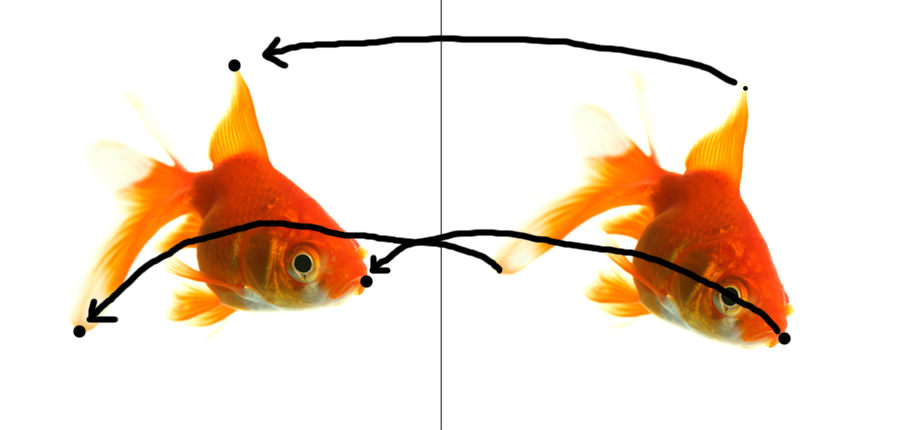
In the case of 3D -3D Rigid Image registration, we have 2 sets of 3 points located in 3D space though prior measurements. In the case of surgery of the human body, we might have 3 small gold markers, known as “fiducial markers” in each 3d image. If our measurements of the marker locations were taken at different times, or with different types of imaging technology, we want to make sure that  we line up the two 3d models as closely as possible, so we can accurately locate the features of interest.

Coordinate systems and rotation in 3D

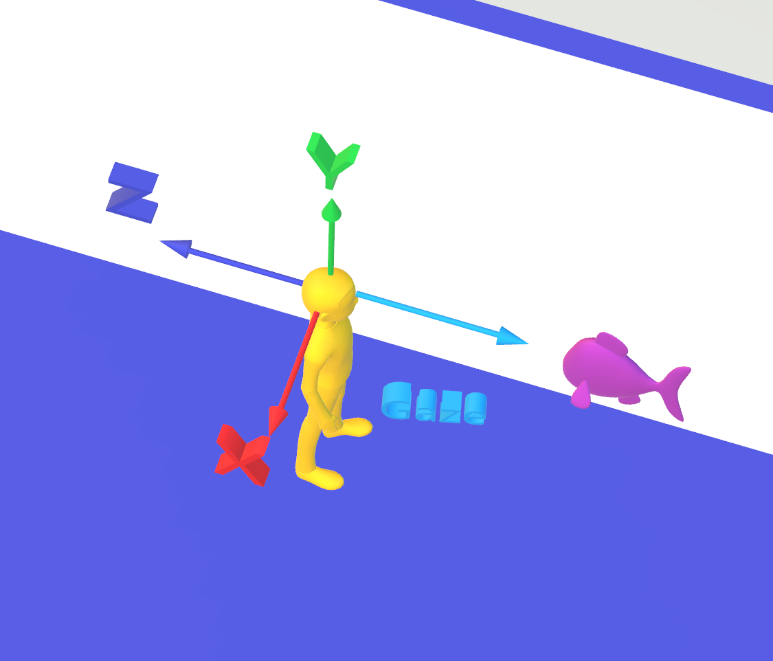
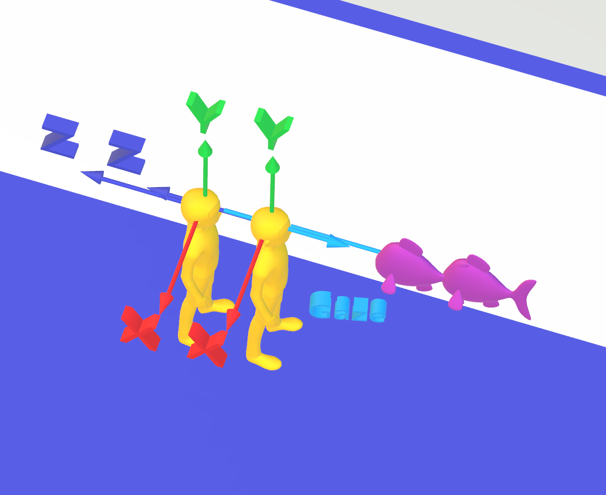
Most people are familiar with 3D coordinates as an extension of the 2D Cartesian coordinate system, by adding a Z axis to the X and Y axis. When rotating points in 3D, it is common and intuitive to think of rotating, for instance, 3 degrees about the X axis, -3 degrees about the Y axis, and 10 degrees about the Z axis.

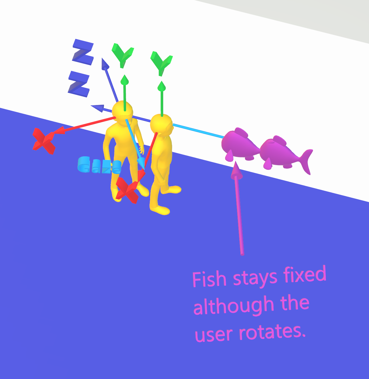
However, there are limitations to this system that are severe enough to lead us to abandon the intuitive approach in favor of something more reliable. One limitation is that the order of the axes that you choose will change the final result – for instance, rotating first about X, then about Y, then about Z, will give a different final result than rotating first about Y, then X, then Z.

In addition, when you rotate at 90 degrees, the math to compute the final results can give ambiguous results.

This representation of rotations in 3D is often referred to as “Euler Angles”. I won’t go into the details of the limitations, but numerous examples can be found online that show the problems with using Euler Angles for computing complex rotational transformations.

One interesting related example happened on the Apollo 11 space craft:

http://en.wikipedia.org/wiki/Gimbal_lock#Gimbal_lock_on_Apollo_11

Quaternions

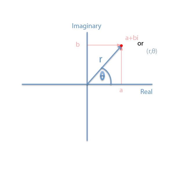
In my previous post we investigated using Complex numbers to make rotations simpler to solve using linear algebra. Quaternions provide us with a very similar advantage  – they allow us to define rotations without the problems of Euler Angles mentioned above, and also provide us with a convenient structure to perform a least squares estimate of the rotation angle.

I won’t go into the details of Quaternions here, but you can find many articles and books that describe their use for defining rotations, especially in software like computer games.

For our purposes, I have written a Matlab class that encapsulates the operations of and on a Quaternion. The Quaternion consists of four member variables – w,x,y  and z. If the w component is set to zero, we have a 3D vector represented within the quaternion – this makes it convenient to mulitply points times quaternions using the same object class.

The problem statement

Source – Hornegger lecture notes, 2011, J. Hornegger, D. Paulus, M. Kowarschik

 

As stated pretty clearly above, the problem we are trying to solve is to find the rotation matrix R that minimizes the squared difference between the measured point
and the original point rotated by R.

Since the rotation matrix R contains sin() and cos() functions, minimizing the equation is not a simple task, and would require an iterative, algorithmic solution. With Quaternions we can create a straightforward set of linear equations.

The rotation by quaternions can be represented as follows:

Recall that the left hand side, p’,  is a quaternion with the w component set to 0. Likewise, on the right hand side we have the original point as quaternion p with it’s w component set to 0. The  character is the quaternion conjugate.

We can factor out the conjugate by multiplying both sides by q:

and the subtract the right side and we are left with

Source – Hornegger lecture notes, 2011, J. Hornegger, D. Paulus, M. Kowarschik

 

The above says we need to find the quaternion q that minimizes the sum of the squared differences between the rotated point (as measured) and the point to be rotated by q.

 

In other words, in a perfect world

we would look for the quaternion q that makes the difference 0, or as close to it as possible.

In linear algebra terms, we’re looking for the nullspace of the matrix.

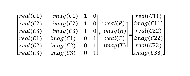
Setting up the matrix

I created a helper function in Matlab

MakeCoefficientMatrix( p, pPrime )

which returns a matrix made from p, the original 3D vector, and pPrime, the rotated vector.

We’re creating the matrix from

(ppPrime* q) – (q * p), so we need to define quaternion multiplication, which is as follows

quat.w = q1.w*q2.w – q1.x*q2.x – q1.y*q2.y – q1.z*q2.z;

quat.x = q1.w*q2.x + q1.x*q2.w + q1.y*q2.z – q1.z*q2.y;

quat.y = q1.w*q2.y + q1.y*q2.w + q1.z*q2.x – q12.x*q2.z;

quat.z = q1.w*q2.z + q1.z*q2.w + q1.x*q2.y – q1.y*q2.x;

So, given the above we can view the matrix as

(ppPrime* q) – (q * p) =

ppPrime.w*q.w – ppPrime.x*q.x – ppPrime.y*q.y – ppPrime.z*q.z – q.w*p.w + q.x*p.x + q.y*p.y + q.z*p.z;

We’re looking for q, so factor q out

q.w(pPrime.w – p.w) – qx(pPrime.x – p.x)  – q.y(pPrime.y – p.y) – q.z(pPrime.z – p.z);
q.w(pPrime.x – p.x)   + q.x(pPrime.w – p.w)  – q.y(pPrime.z   + p.z)  + q.z(pPrime.y + p.y);
q.w(pPrime.y –  p.y) + q.x(pPrime.z + p.z)  + q.y (pPrime.w – p.w) – q.z(pPrime.x  + p.x )
q.w(pPrime.z –  p.z) – q.x(pPrime.y + p.y) + q.y(pPrime.x + q.y)  +   q.z(pPrime.w – p.w);

 

So the complete function is

function [ CM ] = MakeCoefficientMatrix( p, pPrime )

CM = zeros(4,4);

CM(1,1) =  pPrime.w – p.w;

CM(1,2) = -(pPrime.x – p.x);

CM(1,3) = -(pPrime.y – p.y);

CM(1,4) = -(pPrime.z – p.z);

CM(2,1) = pPrime.x – p.x;

CM(2,2) = pPrime.w – p.w;

CM(2,3) = -(pPrime.z + p.z);

CM(2,4) = pPrime.y + p.y;

CM(3,1) = pPrime.y – p.y;

CM(3,2) = pPrime.z + p.z;

CM(3,3) = pPrime.w – p.w;

CM(3,4) = -(pPrime.x + p.x);

CM(4,1) = pPrime.z – p.z;

CM(4,2) = -(pPrime.y + p.y);

CM(4,3) = pPrime.x + p.x;

CM(4,4) = pPrime.w – p.w;

end;

 

Singular Value Decomposition to solve for nullspace

We can make the complete matrix from the 6 points as below, using the helper function:

CM = MakeCoefficientMatrix(p1,pPrime1);

CM2 = MakeCoefficientMatrix(p2,pPrime2);

CM3 = MakeCoefficientMatrix(p3,pPrime3);

% put together

CM = [CM;CM2;CM3];

[U S V] = svd(CM,’econ’);

The singular value decomposition of a matrix is probably one of the most important matrix factorizations to be familiar with. We can use this to find the null space of the matrix, and we can use it to solve other least squares types of matrix computations. The SVD will be a subject of a future blog post.

For now, we take advantage of the fact that the null space of the matrix is in the last column of V:

% get the null space

ns = V(:,4);

qanswer = Quaternion();

qanswer.w = ns(1,1);

qanswer.x = ns(2,1);

qanswer.y = ns(3,1);

qanswer.z = ns(4,1);

and we can check our results by plotting a cross against our rotated objects:

pPrime1 = qanswer * p1 * qanswer.Conjugate();

pPrime2 = qanswer * p2 * qanswer.Conjugate();

plt.PlotVector3WithMarker(pPrime1,pPrime1,’+’,[1 0 0],80,[1 0 0]);

plt.PlotVector3WithMarker(pPrime2,pPrime2,’+’,[1 0 0],80,[1 0 0]);

plt.PlotVector3WithMarker(pPrime3,pPrime3,’+’,[1 0 0],80,[1 0 0]);

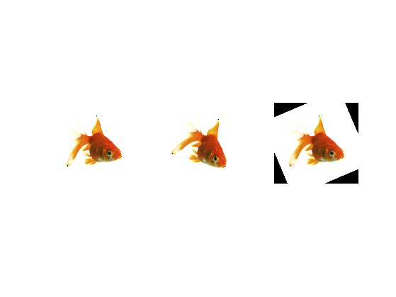
I’ve created a movie showing 3 original spheres, which are then rotated by a random amount (which we don’t “know”),
and then using our method described above we find the angle of rotation and plot a cross hair on our “found” spheres.

3d rotation movie

 

The complete matlab code is below – note, I use my own object-oriented classes, so this code is only a model for your own code, but should be a good example to build from.

 

Rick Frank

 

 

clc;
clear all;
close all;

plt = Plotting();

hold on;
grid on;

colordef black;

% size of our 3d space…

axisVector = [-1.2 1.2 -1.2 1.2 -1.2 1.2];

sphereSize = 0.1;

% Origin and axis for display.

Origin = Vector3(0,0,0);

vAxisX = Vector3(1,0,0);

vAxisY = Vector3(0,1,0);

vAxisZ = Vector3(0,0,1);

% these points are the first measured points.

v1 = Vector3(-0.9,0.2,0.4);

v2 = Vector3(0.8,.9,0.5);

v3 = Vector3(0.4 ,0.4 ,0.3);

red = [1 0 0];
blue = [0 0 1];
green = [0 1  0];

colorX = [1 1 0];
colorY = [0 1 1];
colorZ = [1 0 1];
hold on;

plt.PlotVector3(Origin,vAxisX,’-‘,red);

plt.PlotVector3(Origin,vAxisY,’-‘,blue);

plt.PlotVector3(Origin,vAxisZ,’-‘,green);

plt.PlotSphere(v1,sphereSize,colorX,1.0,axisVector);

plt.PlotSphere(v2,sphereSize,colorY,1.0,axisVector);

plt.PlotSphere(v3,sphereSize,colorZ,1.0,axisVector);

vAxisRotation = Vector3(1,1,1);

d = randi([30,60])

% rotate n degrees about axis….

for n = 1:0.5:d

qr = Quaternion.MakeUnitQuatFromAngleAxis(n,vAxisRotation);

hold off

grid on;
plt.PlotSphere(v1,sphereSize,colorX,1,axisVector);

hold on;

grid on;

plt.PlotSphere(v2,sphereSize,colorY,1,axisVector);

plt.PlotSphere(v3,sphereSize,colorZ,1,axisVector);
p1 = Quaternion.Make3DVecQuat(v1);

%show it

plt.PlotSphere(p1,sphereSize,colorX,1,axisVector);

% rotate it

pPrime1 = qr * p1 * qr.Conjugate();

plt.PlotSphere(pPrime1,sphereSize,colorX,0.2,axisVector);

% another point

p2 = Quaternion.Make3DVecQuat(v2);

plt.PlotSphere(p2,sphereSize,colorY,1,axisVector);

pPrime2 = qr * p2 * qr.Conjugate();

plt.PlotSphere(pPrime2,sphereSize,colorY,0.2,axisVector);

p3 = Quaternion.Make3DVecQuat(v3);

plt.PlotSphere(p3,sphereSize,colorZ,1,axisVector);

pPrime3 = qr * p3 * qr.Conjugate();

plt.PlotSphere(pPrime3,sphereSize,colorZ,0.2,axisVector);

plt.PlotSphere(pPrime1,sphereSize,colorX,0.2,axisVector);

plt.PlotSphere(pPrime2,sphereSize,colorY,0.2,axisVector);

plt.PlotSphere(pPrime3,sphereSize,colorZ,0.2,axisVector);

plt.PlotVector3(Origin,vAxisX,’-‘,red);

plt.PlotVector3(Origin,vAxisY,’-‘,blue);

plt.PlotVector3(Origin,vAxisZ,’-‘,green);

set(gca,’CameraPosition’,[3,-4,-1]);

pause(0.01);

end

%

%(pqPrime1 * q) – (q * p1) = 0;

%(pqPrime2 * q) – (q * p2) = 0;

%etc….

% Utility to create the matrix

%if we add error, then what is the result of the singular values?

ErrorFactor = 0;

pPrime1.AddRandomError(ErrorFactor);

pPrime2.AddRandomError(ErrorFactor);

pPrime3.AddRandomError(ErrorFactor);

CM = MakeCoefficientMatrix(p1,pPrime1);

CM2 = MakeCoefficientMatrix(p2,pPrime2);

CM3 = MakeCoefficientMatrix(p3,pPrime3);

% put together

CM = [CM;CM2;CM3];

[U S V] = svd(CM,’econ’);

 

lastSingularValues = S(:,end);

delta = max(abs(lastSingularValues) – 0);

 

if ((delta > 0.00001) && (delta < 0.01))

disp(‘questionable measurements – adjusting’);

S(:,end) = 0;

newCM = U * S * V’;

[U S V] = svd(newCM);

else if (delta > 2.0e-16)

disp(‘bad measurements – should not be used’);

end

% get the null space

ns = V(:,4);

qanswer = Quaternion();

qanswer.w = ns(1,1);

qanswer.x = ns(2,1);

qanswer.y = ns(3,1);

qanswer.z = ns(4,1);

pause(1.0);

pPrime1 = qanswer * p1 * qanswer.Conjugate();

pPrime2 = qanswer * p2 * qanswer.Conjugate();

plt.PlotVector3WithMarker(pPrime1,pPrime1,’+’,[1 0 0],80,[1 0 0]);

plt.PlotVector3WithMarker(pPrime2,pPrime2,’+’,[1 0 0],80,[1 0 0]);

plt.PlotVector3WithMarker(pPrime3,pPrime3,’+’,[1 0 0],80,[1 0 0]);

 

 

 

 

 

 

 

 

 

 

 

 

 

 

 

 

 

 

I’ve recently been watching the online lectures of Dr. Joachim Hornegger’s Diagnostic Medical Imaging class. For anyone interested in state-of-the-art image processing techniques, especially related to medical imaging, these lectures are extremely useful and also have the side benefit of being entertaining (to geeks, at least).

A link to the course website is here.

What is Image Registration?

Let’s say that you have 2 pictures of the same object, or scene, taken at different times and also from different angles. If you want to see if anything has changed in the object or scene since the time the first picture was taken, it’s much easier if the pictures are lined up so that the object is not rotated, or moved up , down, left, or right. In the medical field, perhaps a tumor has changed over time and you want to align two pictures of the tumor in order to more clearly see any changes that might have taken place over time.

So we want to align the images, but we don’t know the angle or shift between the first and second pictures – and they might have used an x ray device for one image and an MRI for the other. and we must find a way to estimate this angle and/or shift as best as possible.  We can then rotate or shift the picture so that the second picture appears to be in same position and angle as the first. Once this is done you can see the two pictures side by side and compare the object or scene without having to mentally rotate or shift the image.

So, let’s look at some pictures. Here we have a picture of a goldfish, and then we have the same goldfish, but rotated by some number of degrees clockwise. How can we figure out what we need to do to get the second image to align back up with the first?

 

Point Correspondences

One way to make the image registration easier is to provide hints to the algorithm. A human can manually locate points in both images that are the “same” points in the two objects. You can see the black spots I placed on the fish images above. Once we have placed the corresponding points, we must then compute the transformation that takes us from picture 2 back to picture 1:

 

 

Note, the pictures above have selected points that look like they are in 3d, but in this example we just want to line up the fish in 2 dimensions. So we treat the spots as just 2d points, with an x coordinate and a y coordinate.

Imagine, a use for imaginary numbers!

You probably learned about imaginary, a.k.a complex,  numbers in middle or high school, and at that time like most people I had very little idea of what use they might be. It just seemed to me to be one more kooky thing I had to remember for a test. It turns out, however, that there are actually many uses for them in practical applications. One of those uses is that they make finding the image registration parameters we need for our above problem relatively easy to obtain.

Professor Hornegger covers the details of the 2D-2D image transform using complex numbers quite thoroughly in the lecture and the lecture slides. I will go through the steps involved and also implement some Matlab code to perform the 2D – 2D Image Registration. What about 3D-3D, as mentioned in the title? Well we’ll get to that in part 2…

Complex numbers make things simple?

The useful thing about complex numbers for our situation is that they can be used for rotating points. Multiplying a complex number by another complex number results in a rotation and scaling of the first number by the second. If we create our complex number carefully, (by having it’s magnitude be 1.0) we can eliminate the scaling and just have the rotation.

Complex numbers have a “real” part and an “imaginary” part. We can plot these on a graph by having the x axis be for the “real part” and the y axis for the imaginary part of the complex number.

 

In the diagram above we see a red point that is described uniquely by two different coordinate representations. In the pink color, we see the complex number representation, and in the light blue color we see the polar representation, where the point can be uniquely described by the line length r and the rotation angle theta.

Diversion – deriving Euler’s Identity

Now we can set up some handy equivalencies, by noting the following:

a = r * cos(Θ)
b = r *  sin(Θ)

So, we have

a + bi = r * cos(Θ) + r*i*sin(Θ) = r( cos(Θ) +i*sin(Θ))

For our purposes, we want to deal with only rotations, and no scaling. So, we limit our value of r to 1.0. This lets us take out the r, since it would be only  a multiplication by 1.0.

a+bi = cos(Θ) + i*sin(Θ) or, if we create a new single letter for  a + bi, let’s call it z, we can say

z = cos(Θ) + i*sin(Θ).

We can then take the derivative of this function of Θ, and we end up with

dz/d theta = -sin(Θ) + i*cos(Θ)

and then factoring out the i gives us

dz/d Θ = i(i*sin(Θ) + cos(Θ)).

This looks familiar – if we rearrange the right hand side we get

dz/d Θ = i(cos(Θ) + i*sin(Θ)), which is = i(z)!

So, dz/d Θ = i(z).

To solve this, let’s move the z’s to the same side, giving

dz/z = d Θ * i

Solving by integrating both sides give

ln(z) = Θ * i

exponentiating, that is making each side the exponent of the base e, gives

z = e ^ Θ*i

Now we have yet another way of representing complex numbers, using the constant e raised to the Θ  i power.

This form is sometimes called the Euler form.

So what have we shown? Well, given the Euler representation of our complex number, of unit length, we can see that multiplying two complex numbers gives a rotation:

a = e^Θ[1] * i  * e^Θ[2] * i = e^(Θ[1] + Θ[2])i as seen here:

 

Above we see a complex point, represented by a unit length and 45 degree angle, multiplied by itself, giving a rotation of 45 degrees CCW. This demonstrates the idea that multiplying complex numbers provides us with an “easy” way to rotate points.

How does all this help us solve our problem with the fishes?

A rotation and translation of points can be described as below:

 

Here we see that we have a rotation matrix, R, that has Cos and Sin functions. To get the “best” answer, we want to minimize the sum of the squared differences between the rotatedPoint and the originalPoint rotated by Θ and translated by t. This give us the “best” answer, however the Cos and Sin functions make the problem non-linear, and that is not desired, because the solution will be difficult to compute.

By using the complex numbers this way we can set up a system of linear equations, which provides us a very straightforward way to solve for the unknown rotation and translation parameters.

 

We can set up this kind of equation with the complex numbers as follows:

C1  = unrotated complex point 1
C2 =  unrotated complex point 2
C3 =  unrotated complex point 3

C11 = rotated complex point 1
C22 = rotated complex point 2
C33 = rotated complex point 3

 

 

This matrix is the usual Ax = b system of linear equations. We can solved this for x in Matlab with the handy backslash operator, i.e. x = A\b.

Recall we are looking for the complex number R, which will be our rotation, and T which is our translation. These two complex numbers make up the vector x above.

So, we will have the following matrix to solve:

Let’s look at some code. Note, the matlab code below uses object oriented classes of my own design that wrap complex numbers, vectors, etc. However, the reader should be able to create similar classes to get the same results. I prefer the object oriented flavor of the code over the procedural flavor of matlab out of the box, so to speak.

%set up and read in the fishes...

clc;

clear all;

close all;

I1 = imread('Fish.png');

I2 = imread('Fish2.png');

subplot(1,2,1);

imshow(I1);

subplot(1,2,2);

imshow(I2);

%the point correspondences - these are the human selected points.

p1 = [267,79];

p2 = [96,372];

p3 = [413,318];

p11 = [329,98];

p22 = [56,301];

p33 = [370,375];

[imR imC] = size(I1);

%NOTE, the image points are in "image coordinates, with (1,1) at top left.

% We flip these into cartesion form, with (0,0) in the bottom left.

p1 = imCoords2cartCoords(imR,p1);

p2 = imCoords2cartCoords(imR,p2);

p3 = imCoords2cartCoords(imR,p3);

p11 = imCoords2cartCoords(imR,p11);

p22 = imCoords2cartCoords(imR,p22);

p33 = imCoords2cartCoords(imR,p33);

% Create our objects, from real and imaginary axis points.

% these are the original points...

c1 = Complex(p1(1,1),p1(1,2));

c2 = Complex(p2(1,1),p2(1,2));

c3 = Complex(p3(1,1),p3(1,2));

% these are the rotated points...

c11 = Complex(p11(1,1),p11(1,2));

c22 = Complex(p22(1,1),p22(1,2));

c33 = Complex(p33(1,1),p33(1,2));

% create our custom object oriented plotting object...

plt = Plotting();

figure;

%draw the points....

plt.PlotComplex(c1,'O',[1 0 1],10,[1 0 1]);

hold on;

plt.PlotComplex(c2,'O',[1 1 0],10,[1 1 0]);

plt.PlotComplex(c3,'O',[0 1 1],10,[0 1 1]);

plt.PlotComplex(c11,'O',[1 0 0],10,[1 0 0]);

plt.PlotComplex(c22,'O',[0 1 0],10,[0 1 0]);

plt.PlotComplex(c33,'O',[0 0 1],10,[0 0 1]);

% Create the "A" matrix......

A = zeros(6,4);

A(1,1) = real(c1.c);

A(1,2) = -imag(c1.c);

A(2,1) = real(c2.c);

A(2,2) = -imag(c2.c);

A(3,1) = real(c3.c);

A(3,2) = -imag(c3.c);

A(1,3) = 1;

A(2,3) = 1;

A(3,3) = 1;

A(4,1) = imag(c1.c);

A(4,2) = real(c1.c);

A(5,1) = imag(c2.c);

A(5,2) = real(c2.c);

A(6,1) = imag(c3.c);

A(6,2) = real(c3.c);

A(4,4) = 1;

A(5,4) = 1;

A(6,4) = 1;

b = zeros(6,1);

% Set up the b matrix.....

b(1,1) = real(c11.c);

b(2,1) = real(c22.c);

b(3,1) = real(c33.c);

b(4,1) = imag(c11.c);

b(5,1) = imag(c22.c);

b(6,1) = imag(c33.c);

%SOLVE for X =

x = A\b

% the x vector now has r, and t...

r = Complex(x(1,1),x(2,1));

% just out of curiousity, display the angle, and the length of r

angleDegrees = r.angle() * 180/pi;

disp(angleDegrees);

disp(r.length());

% rotate our image....

I3 = imrotate(I2,angleDegrees,'bilinear','crop');

figure;

% and display it....

subplot(1,3,1);

imshow(I1);

subplot(1,3,2);

imshow(I2);

subplot(1,3,3);

imshow(I3);

So, the final result are seen below. The images are from left to right, the original, the rotated, and the registered image. Note that rotating the image creates a black background where the pixels are not in the original.

 

It turns out that the fish was rotated approximately 23 degrees…..

 

Next up in part 2……3d – 3d rotations with Quaternions….

Rick Frank

 

 

 

 

 

In the first part of this series we discussed first order edge enhancement, and how we looked for changes in the image to determine where an edge was located. To find these changes, we looked at the an approximation of the first derivative – (the rate of change) – over sections of the image. We approximated the first derivative with a centered difference equation.

We only touched on a few basic concepts, so, there’s quite a bit more that could be covered on first derivative edge enhancement. There are a number of good books now to explore these concepts – I’ll reference them at the end of this post.

Let’s move on to second order edge enhancement.

To review, the problem we have at hand is trying to enhance the “edges” in an image. When you zoom in on an image on a computer screen, you soon see that the image is actually composed of  pixels – dots –  it’s only when we “stand back” from the image that we see the image clearly. It’s a bit like French Impressionist paintings.

Too simplify our understanding of the image and how we process it, we can turn our gray image on its side, and look at if from the “edge”. We can then select just one row of pixels and think about it in one dimension. If we assign each pixel in our row a height based on the gray value, we end up with sort of a bar chart:We can think of the row of pixels this way as a function, with the height as the y value and the pixel number in the row as the x value.

So that is how our data in the image looks from the side, in one dimension. It’s an approximation of a function. Now, let’s look a little bit at the abstract concepts. We’ll fire up the excellent Graphing Calculator (from Pacific Tech – http://www.pacifict.com) to take a look at some concepts. First, let’s create a theoretical edge. We can use the logistic “S” function to create what could be considered a smooth edge:

Here we see a theoretical edge – in reality the edge would be more like our previous bar chart, but for now we’ll just stay in the continuous world.

Recall from the first post in this series that the estimated derivative of this function can be approximated with a centered difference equation. Let’s try it:

This looks correct – the green curve estimates the rate of change of the red curve. That rate is fastest where the green curve reaches it’s peak, and then slows back to zero as the red curve settles on the top edge.

If we create an image from the first derivative, we see that it would place an edge pixel right in the middle of our curve. This is not a bad estimate, but it may not be quite what we want, or expect. Imagine that the left side of the red curve are all dark pixels, and then the image quickly jumps up to white pixels on the right. Our eye would most likely measure the edge at the top of the red curve, not in the middle. We would be drawn to where the end of the flat bright surface “stops”.

If that’s our desire, then let’s see what taking the second derivative might offer us.

We can approximate the second derivative in a way similar to how we estimated the first derivative, and see what it looks like against our “edge”. The second derivative is the derivative of the derivative – and a good way to approximate that is by taking the difference of differences – The difference of a forward difference and a backward difference:

Here we have a forward difference minus a backward difference, all divided by stepsize. In our case, our stepsize is 1 (pixel) so we can just take out all the denominators. Now, we have our second derivative estimate in the yellow curve below. How could we use this to help us find an edge?

If we look at our equation, we can recall from the first post that we can make a “kernel” and apply it to the image by multiplying and summing as we move across the image. What would our kernel be from this equation? First let’s simplify the function k(a) a bit.

Above we have now made the function describing the yellow curve to be 1 of the pixel ahead, (f( a + ), – 2 of the pixel we are on, -2(f a) + 1 or the pixel behind us – + 1f(a-a).

Recall from Part of one this article that we can create a “Kernel” to describe the coefficients of the equation above. In this case the one dimensional kernel would be

1 -2 1
If we see the yellow curve as our resulting edge  enhanced image, i.e.  the image after the kernel is applied, we can see that the first part of the curve has a positive value, and shows what you might consider the start of the edge. The second half of the curve has negative values, and it lines up more or less where the edge is fully begun. Where the yellow curve crosses zero on the y axis – the “zero
crossing” is right between the two. This gives us a “start” of the edge even further from the edge that the first derivative found! What to do.

It would seem that a practical place to locate the edge is where the edge is really begun in full, but, our resulting image based on our yellow curve would have negative coefficients, which would de-emphasize the edge we want –  not very useful. What we can do, however, is flip the curve over. Let’s reverse the signs and take a look:

Notice that our kernel is now -1 2 -1. And the right half of the yellow curve pushes up just where the “edge” is beginning to fully
emerge. That’s closer to what we would perceive visually as the edge, where the white pixels meet the black pixels. in addition, the negative coefficients will de-emphasize what we don’t want perceived as the edge, so as to add further contrast to our image.

Let’s run the following filter on our test image

0 0 0
-1 2 -1
0 0 0

Here’s the original image again:

This is a bit dim, but the vertical lines do get enhanced quite nicely. Let’s pull in some diagonal lines – note, we have to balance the positive numbers and the negative coefficients, since we are keeping the pixel at the center of the kernel. So, the center coefficient has to balance the negatives, and in this case that means it must be 4:

0 0 -1
-1 4 -1
-1 0 –

Now let’s pull in the other diagonals:

-1 0 -1
-1 6 -1
-1 0 -1

Now let’s fill out the kernel completely:

-1 -1 -1
-1 8 -1
-1 -1 -1

These filters do a nice job of enhancing the edges. This filter is often called a “Laplacian” filter.

Some excellent books for further reading on these topics are:

Digital Image Processing (3rd Edition) [Hardcover]
Rafael C. Gonzalez  Richard E. Woods

The Image Processing Handbook, Fifth Edition by John C. Russ

Hope you found these posts interesting and also perhaps useful!

Rick Frank
Dominion Software, Inc.
rfrank@dominionsw.com