
Image Recognition with the Matlab Deep Learning Toolbox
After some time in the Artificial Intelligence Doghouse, Neural Networks regained status after Alex Krizhevsky, Ilya Sustkever, and Goeffrey Hinton won the Large Scale Visual Recognition Challenge in 2012 using their Neural Network, now known as AlexNet.
Details can be found in their paper.
The Matlab Deep Learning Toolbox makes it really easy to develop our own Deep Learning network to use for our tree seedling classification task. And, as it turns out, we can take advantage of the work done by the winners above by using their trained network to bootstrap our own network using a technique called Transfer Learning.
Overview of Deep Learning Neural Networks
A Neural Network is designed to mimic the way a biological neuron “Activates” on a given stimulus. How close it comes to recreating an actual biological neuron I will leave to the Neuroscientists to decide. But that is the concept. These neurons are then connected into “Layers”. The “Deep” part of “Deep Learning” refers to the fact that there are many layers of neurons in a particular network, therefore creating a “Deep” Neural Network.
Let’s take a look at the typical diagram for a section of a Neural Network:

The circles on the left are the activations. The lines connecting to the circle on the right are the weights. The circle on the right is the output which is the weighted sum of the activations plus a bias, b, plugged in as a parameter to σ(), which is a function known as a Rectifier which simply sets everything < 0 to 0. We’ll skip over the bias and the sigma function, as they are important but not essential to the basic concept.
These diagrams certainly didn’t mean all that much to me at first; as a programmer, I immediately thought “what does this look like in code”?
Well, it turns out that if you know a bit about image processing filters, it is easy to understand the basic concepts of convolutional neural networks.
It turns out that for the image specific tasks, like classifying photos, the activations are the input pixels. The weights are the values in an image filter. So, for instance, a filter could be a 3 by 3 edge detection filter,
| -1 | 0 | 1 |
| -1 | 0 | 1 |
| -1 | 0 | 1 |
or any other type of image filter. The activations are the pixels of the input image, and so one is left with the “classic” image processing task of sliding a filter across an image, taking the dot product and setting a new pixel – potentially a new activation in the next layer.

Now, here’s where the “Learning” part of Deep Learning comes in. Instead of first specifying what filters to use, we tell the network what result we want, and it keeps adjusting the filters until it gets that result, or close to it. This feedback is known as back-propagation. So, let’s say we want to train the network to recognize an image with the label “Cat”. We keep feeding the images we want to be recognized as a Cat, and the algorithm keeps updating the filters until they agree that the images can be classified as a Cat. This is a bit of a simplification, but it is the basic essence of what is happening during the training process.
Once the network is trained properly, the filters will then be able to process an unseen before image as a “Cat”. 
With Matlab, we can actually look at the filters in the first layer of AlexNet.
Load AlexNet
net = alexnet;
Let’s look at the Layers:
net.Layers
ans =
  25x1 Layer array with layers:

     1   'data'     Image Input                   227x227x3 images with 'zerocenter' normalization
     2   'conv1'    Convolution                   96 11x11x3 convolutions with stride [4  4] and padding [0  0  0  0]
     3   'relu1'    ReLU                          ReLU
     4   'norm1'    Cross Channel Normalization   cross channel normalization with 5 channels per element
     5   'pool1'    Max Pooling                   3x3 max pooling with stride [2  2] and padding [0  0  0  0]
     6   'conv2'    Convolution                   256 5x5x48 convolutions with stride [1  1] and padding [2  2  2  2]
     7   'relu2'    ReLU                          ReLU
     8   'norm2'    Cross Channel Normalization   cross channel normalization with 5 channels per element
     9   'pool2'    Max Pooling                   3x3 max pooling with stride [2  2] and padding [0  0  0  0]
    10   'conv3'    Convolution                   384 3x3x256 convolutions with stride [1  1] and padding [1  1  1  1]
    11   'relu3'    ReLU                          ReLU
    12   'conv4'    Convolution                   384 3x3x192 convolutions with stride [1  1] and padding [1  1  1  1]
    13   'relu4'    ReLU                          ReLU
    14   'conv5'    Convolution                   256 3x3x192 convolutions with stride [1  1] and padding [1  1  1  1]
    15   'relu5'    ReLU                          ReLU
    16   'pool5'    Max Pooling                   3x3 max pooling with stride [2  2] and padding [0  0  0  0]
    17   'fc6'      Fully Connected               4096 fully connected layer
    18   'relu6'    ReLU                          ReLU
    19   'drop6'    Dropout                       50% dropout
    20   'fc7'      Fully Connected               4096 fully connected layer
    21   'relu7'    ReLU                          ReLU
    22   'drop7'    Dropout                       50% dropout
    23   'fc8'      Fully Connected               1000 fully connected layer
    24   'prob'     Softmax                       softmax
    25   'output'   Classification Output         crossentropyex with 'tench' and 999 other classes
We can take a look at the 2nd layer and visualize the image filters. There are 96 filters, 11 pixels by 11 pixels by 3 pixels (one set of pixels each for R, G, B colors).
We offset the pixels all into the positive range so we can see them more easily, then write them as a tiff file.
layer = net.Layers(2);
img = imtile(layer.Weights);
mn = min(min(min(img)));
img = img - mn;

imgu = uint8(img.*255);

imwrite(imgu,'Tiles.tif','tif');

This is pretty interesting. 96 image filters that were “learned” from the 1.2 million images with 1000 different labels. I also notice the cyan and green colors, which remind me of the Lab color space from a previous post.
There a lot of details that one can go into here, of course. We’ll skip ahead to how we can use this network to recognize our own images.
Transfer Learning
It turns out that we can retrain an existing network to classify our seedlings using what is known as “Transfer Learning”. Using the Matlab Deep Learning Toolbox, we can do this by replacing two of the layers in the original AlexNet with our own.
First, we load the network, and set up a path to our Labeled image folders.
net = alexnet;
imagePath = 'C:\Users\rickf\Google Drive\Greenstand\TestingAndTraining';
We can set up our datastore, and use a Matlab helper function to pick 80 percent of the images for training. In addition, the augmentedImageDatastore() function let’s us scale the images to the required 227×227 inputs that AlexNet requires.
imds = imageDatastore(imagePath,'IncludeSubfolders',true,'LabelSource','foldernames');
[trainIm, testIm] = splitEachLabel(imds, 0.8,'randomized')

trainData = augmentedImageDatastore([227 227], trainIm)
testData = augmentedImageDatastore([227 227], testIm)
If we look above we can see that the final layers in the AlexNet network are set up for 1000 different labels.
23 'fc8' Fully Connected 1000 fully connected layer
24 'prob' Softmax softmax
25 'output' Classification Output crossentropyex with 'tench' and 999 other classes
What we need to do is to replace layer 23 with a fully connected 6 input layer (for our 6 labels),
and replace 25 with a new classifier that will accept those 6 inputs from the softmax layer.
layer(23) = fullyConnectedLayer(6,'Name','fcfinal');
layer(end) = classificationLayer('Name','treeClassification');
opts = trainingOptions('adam','InitialLearnRate',0.0001,'Plots','training-progress','MaxEpochs',10);
[net,info] = trainNetwork(trainData,layer,opts);
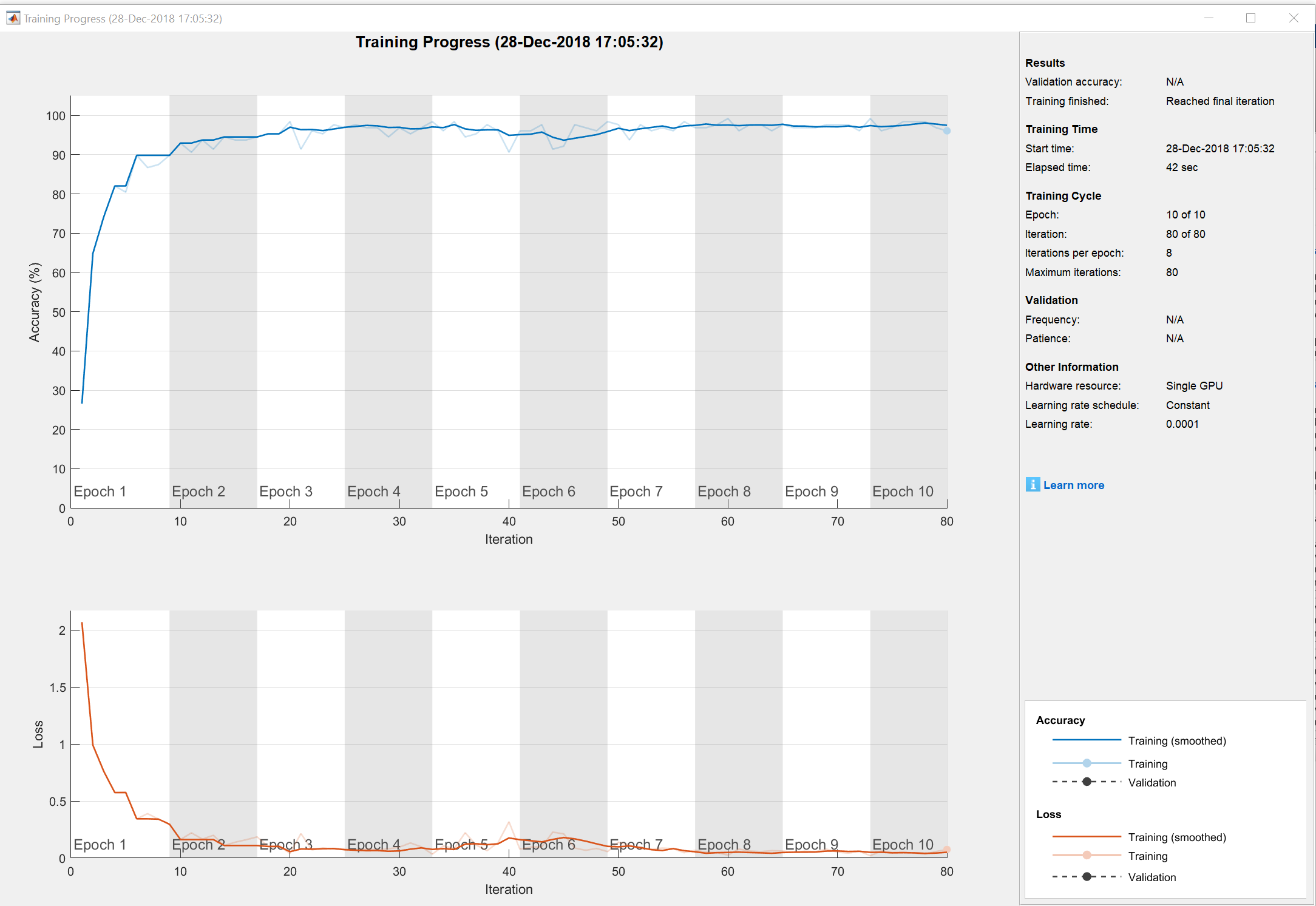
We specified the option to plot progress, which is shown above.
The final results can be seen in our confusion matrix.
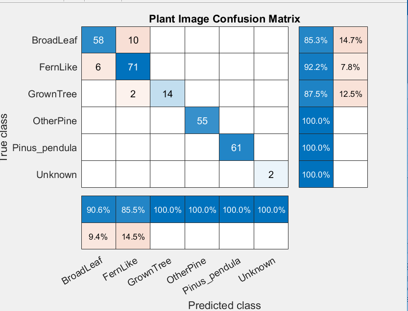
Much better results that the Support Vector Machine, and no color segmentation was needed!
I would suspect with more training data we can get the Broadleaf and Fernlike classifications to improve. We’ll try that, and then put the network to a test of classifying unseen new images in the next post.