In the first part of this series we discussed first order edge enhancement, and how we looked for changes in the image to determine where an edge was located. To find these changes, we looked at the an approximation of the first derivative – (the rate of change) – over sections of the image. We approximated the first derivative with a centered difference equation.
We only touched on a few basic concepts, so, there’s quite a bit more that could be covered on first derivative edge enhancement. There are a number of good books now to explore these concepts – I’ll reference them at the end of this post.
Let’s move on to second order edge enhancement.
To review, the problem we have at hand is trying to enhance the “edges” in an image. When you zoom in on an image on a computer screen, you soon see that the image is actually composed of pixels – dots – it’s only when we “stand back” from the image that we see the image clearly. It’s a bit like French Impressionist paintings.
Too simplify our understanding of the image and how we process it, we can turn our gray image on its side, and look at if from the “edge”. We can then select just one row of pixels and think about it in one dimension. If we assign each pixel in our row a height based on the gray value, we end up with sort of a bar chart: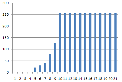 We can think of the row of pixels this way as a function, with the height as the y value and the pixel number in the row as the x value.
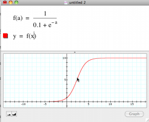
So that is how our data in the image looks from the side, in one dimension. It’s an approximation of a function. Now, let’s look a little bit at the abstract concepts. We’ll fire up the excellent Graphing Calculator (from Pacific Tech – http://www.pacifict.com) to take a look at some concepts. First, let’s create a theoretical edge. We can use the logistic “S” function to create what could be considered a smooth edge:
Here we see a theoretical edge – in reality the edge would be more like our previous bar chart, but for now we’ll just stay in the continuous world.
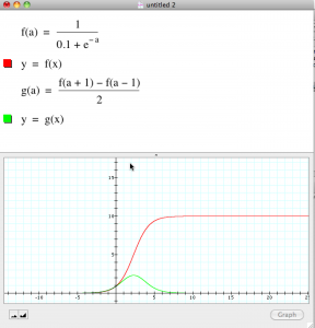
Recall from the first post in this series that the estimated derivative of this function can be approximated with a centered difference equation. Let’s try it:
This looks correct – the green curve estimates the rate of change of the red curve. That rate is fastest where the green curve reaches it’s peak, and then slows back to zero as the red curve settles on the top edge.
If we create an image from the first derivative, we see that it would place an edge pixel right in the middle of our curve. This is not a bad estimate, but it may not be quite what we want, or expect. Imagine that the left side of the red curve are all dark pixels, and then the image quickly jumps up to white pixels on the right. Our eye would most likely measure the edge at the top of the red curve, not in the middle. We would be drawn to where the end of the flat bright surface “stops”.
If that’s our desire, then let’s see what taking the second derivative might offer us.
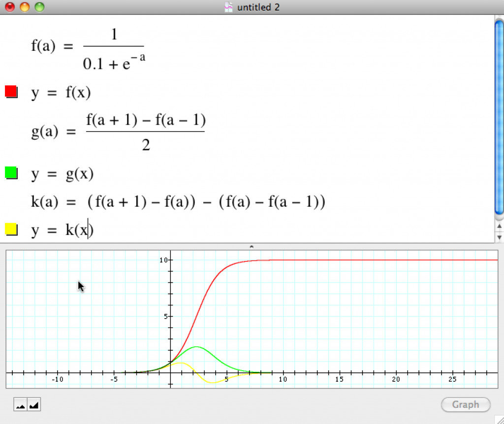
We can approximate the second derivative in a way similar to how we estimated the first derivative, and see what it looks like against our “edge”. The second derivative is the derivative of the derivative – and a good way to approximate that is by taking the difference of differences – The difference of a forward difference and a backward difference:
 Here we have a forward difference minus a backward difference, all divided by stepsize. In our case, our stepsize is 1 (pixel) so we can just take out all the denominators. Now, we have our second derivative estimate in the yellow curve below. How could we use this to help us find an edge?
If we look at our equation, we can recall from the first post that we can make a “kernel” and apply it to the image by multiplying and summing as we move across the image. What would our kernel be from this equation? First let’s simplify the function k(a) a bit.
Above we have now made the function describing the yellow curve to be 1 of the pixel ahead, (f( a + ), – 2 of the pixel we are on, -2(f a) + 1 or the pixel behind us – + 1f(a-a).
Recall from Part of one this article that we can create a “Kernel” to describe the coefficients of the equation above. In this case the one dimensional kernel would be
1 -2 1
If we see the yellow curve as our resulting edge enhanced image, i.e. the image after the kernel is applied, we can see that the first part of the curve has a positive value, and shows what you might consider the start of the edge. The second half of the curve has negative values, and it lines up more or less where the edge is fully begun. Where the yellow curve crosses zero on the y axis – the “zero
crossing” is right between the two. This gives us a “start” of the edge even further from the edge that the first derivative found! What to do.
It would seem that a practical place to locate the edge is where the edge is really begun in full, but, our resulting image based on our yellow curve would have negative coefficients, which would de-emphasize the edge we want – not very useful. What we can do, however, is flip the curve over. Let’s reverse the signs and take a look:
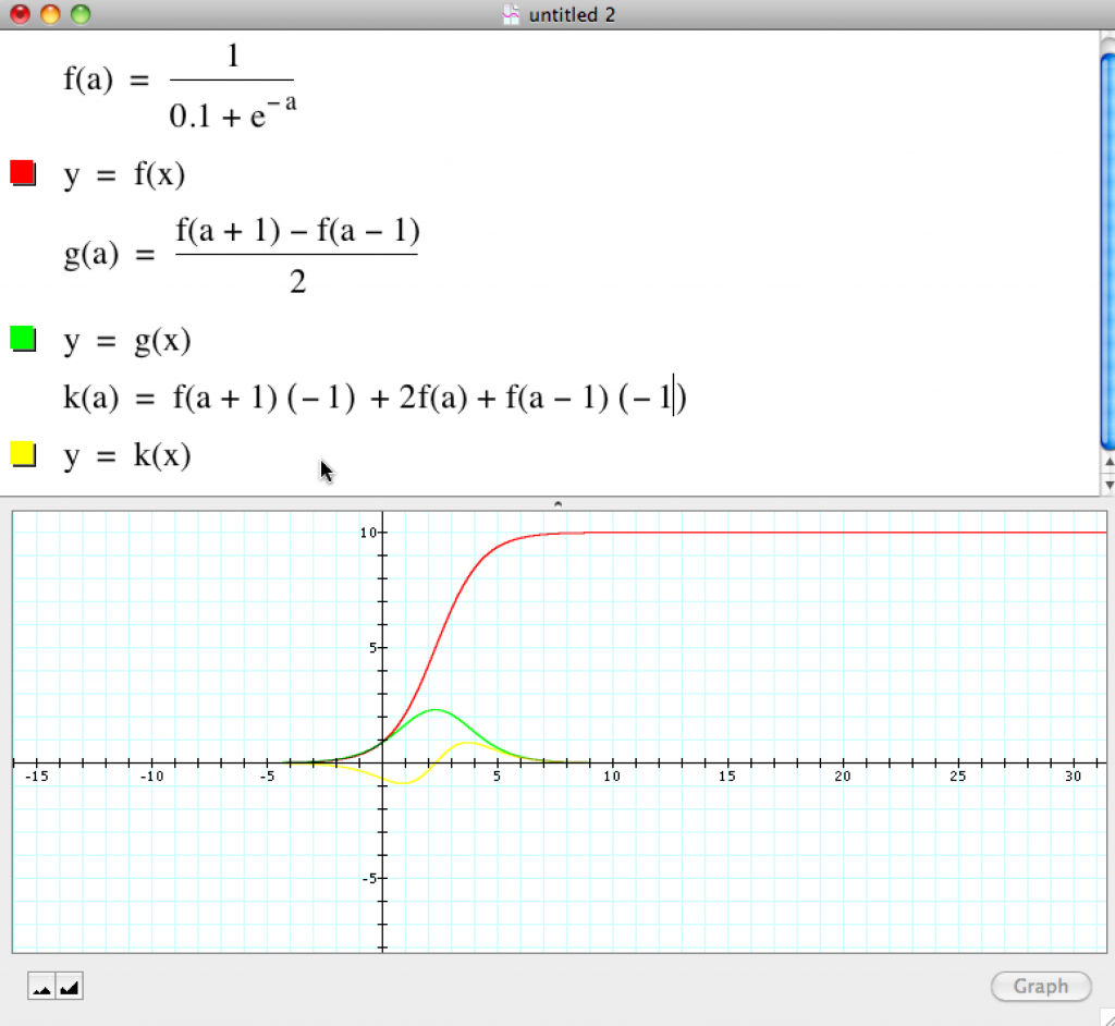 Notice that our kernel is now -1 2 -1. And the right half of the yellow curve pushes up just where the “edge” is beginning to fully
emerge. That’s closer to what we would perceive visually as the edge, where the white pixels meet the black pixels. in addition, the negative coefficients will de-emphasize what we don’t want perceived as the edge, so as to add further contrast to our image.
Let’s run the following filter on our test image
0 0 0
-1 2 -1
0 0 0
Here’s the original image again:
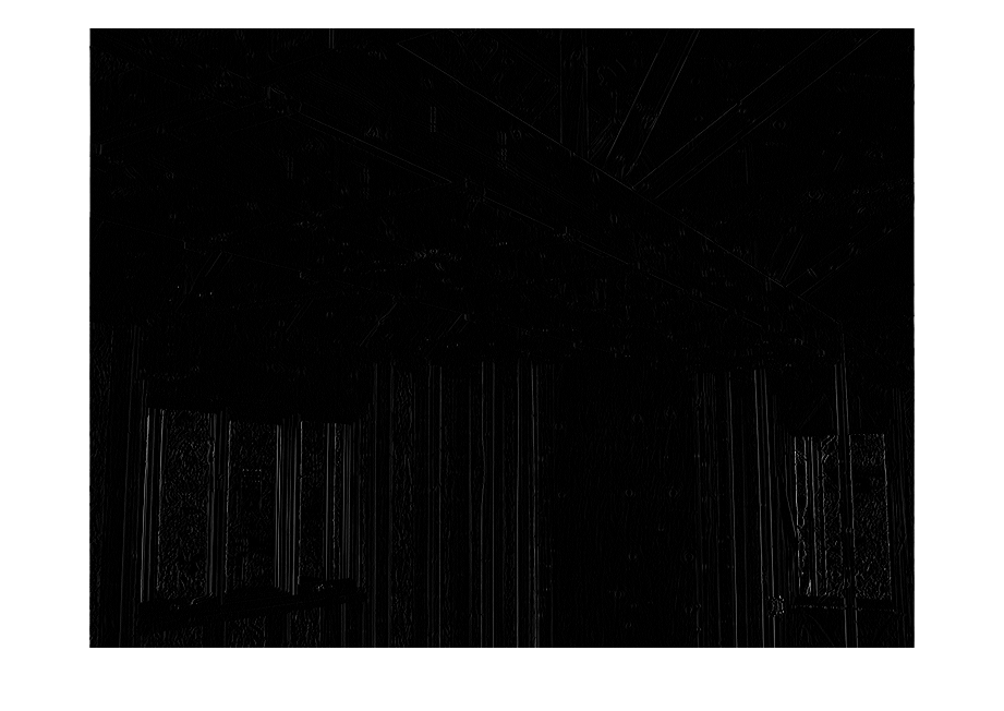 This is a bit dim, but the vertical lines do get enhanced quite nicely. Let’s pull in some diagonal lines – note, we have to balance the positive numbers and the negative coefficients, since we are keeping the pixel at the center of the kernel. So, the center coefficient has to balance the negatives, and in this case that means it must be 4:
0 0 -1
-1 4 -1
-1 0 –
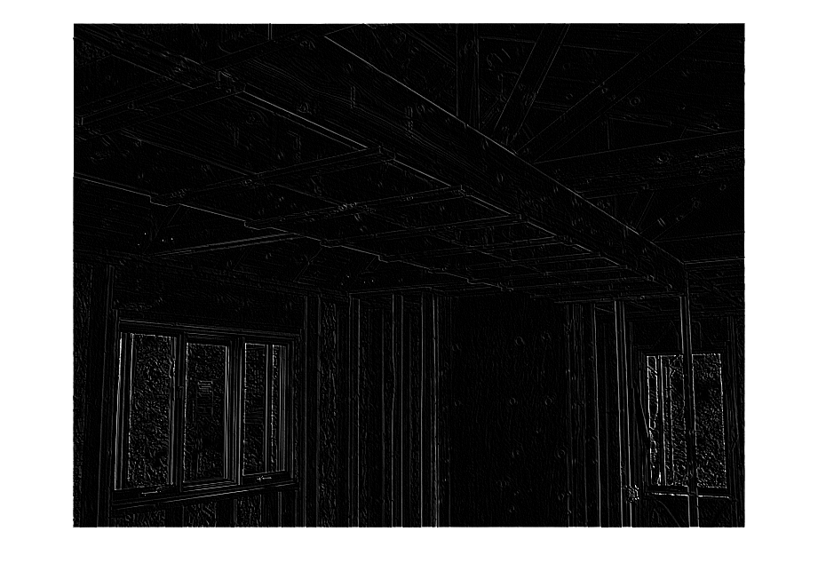 Now let’s pull in the other diagonals:
-1 0 -1
-1 6 -1
-1 0 -1
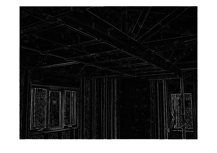 Now let’s fill out the kernel completely:
-1 -1 -1
-1 8 -1
-1 -1 -1
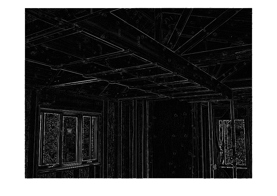 These filters do a nice job of enhancing the edges. This filter is often called a “Laplacian” filter.
Some excellent books for further reading on these topics are:
Digital Image Processing (3rd Edition) [Hardcover]
Rafael C. Gonzalez Richard E. Woods
The Image Processing Handbook, Fifth Edition by John C. Russ
Hope you found these posts interesting and also perhaps useful!
Rick Frank
Dominion Software, Inc.
rfrank@dominionsw.com
