If you’ve done a bit of image processing, or read about it, you’ve probably run into the concept of “edge detection”. In the first part of this article I’ll take a closer look at the basics of edge detection, and explore in more detail what’s going on in those little boxes of numbers.

When people hear of the concept  of edge detection in images, they sometimes think of  finding objects in images, and obtaining the actual coordinates of the objects in the image. However, the various algorithms called edge “detection” would  probably better be called edge “enhancement”. These algorithms amplify or mark where the segments in an image change, and the result is a new image showing the location of these changes, which are “edges” in the image. So, the “detection” part does not include creating a map of coordinates of various regions – other algorithms are needed for this task. However, edge detection is a useful tool in preparing images for location detection, and for enhancing the lines, edges, and corners in images for other image processing tasks.

If we start with a very simple example, it is easier to understand the basic idea for edge enhancement. Here we have an image with a single, simple edge, where the white section meets the black section in the middle:

We will use the convention that the value of the color black on the left is 0, and the value of the white on the right is 1.  Let’s take this image down to 1 dimension, and look at it from the edge:

Here we can see the black area as all zeros, and the white area as all ones. To detect where that change happens, we have to bring in the dreaded “C” word, Calculus.  But, we really only need to know a bit about that topic to understand how to find the edge of the image.

We are looking for a change – a difference – in the image. We want to note where those differences occur. The ideas of Calculus help us find this difference. We can move along the data from left to right, on step at a time, looking for these changes.

To be clear, we have a discontinuous function,  as seen by the big jump between 0 and 1. Calculus doesn’t like to deal with this type of data. However, we are in the computer world,  where we always have to deal with these types of discontinuities between values.

The concepts we will borrow from the Calculus are the idea of derivatives, which is the rate of change, and the concept of the limit of the size of the step as it approaches zero.  The rate of change is how fast our data is changing – how much change vs how many steps. – The concept of the limit of the step size is simply taking the step size to its smallest theoretical value, which gives us the most accurate measurement. In our computer world, we have a simpler model – our step size in this case is just 1 pixel,  and as we step across this data we can estimate the rate of the change across  small sections of our data. This concept is known as Finite Differences, and since our world inside the computer has finite steps and step sizes, we will use this concept.

Imagine walking along inside a building, writing down the difference in your position vertically in the building as you walk.  As you start to walk your position is 0 feet off the floor, and you look ahead and measure the difference between where you are and where you will be the next step forward. As you move along the floor for four steps, say, you note at each step that there is no difference in the height between where you are and where you will be, so you write down a 0 difference for that step. Then you reach a stair, and you look forward and measure the difference between the height of the  first stair and the floor. Let’s say it’s 1 foot. The difference is 1 (where you will be) – 0 (where you are now). So you write 1 down and then take a step.  The floor is level after this first step  and so as you continue along there is no change in your vertical position, so you write down zeros.  So, now your notebook has something like the following written in it:

0 0 0 0 1 0 0 0 0

Congratulations! You detected the edge in the floor in the building! I hope you didn’t trip over it.

In more mathematical terms, you’ve taken the “Forward Difference” of the data along your path. This can be written as:

Height(where you are + 1) – Height(where you are)/Step Size

Here, our step size is conveniently just “1” step, so we can just pay attention to the top part of the fraction.

It turns out, however, that this method is not quite as accurate as it could be. If you are measuring a surface that has a rapidly changing shape, rather than our simple floor,  your measurements of the change will be limited by the size of your step.  Using our walking example, you could improve your estimate if as you go along you stop and look forward,  and then staying where you are look backwards, and then average these two measurements. This is known as a “Centered Difference”, and it is a bit intuitive that this kind of measurement might be a better estimate. It’s like the phrase “splitting the difference.”

Height(where you are + 1) – Height(where you are – 1)/2 x Step Size

There is also a “Backward Difference”, which as you can imagine takes the measurement where you are and the measurement in back of you and takes the difference between them. These Finite Differences provide an estimate of the first derivative of our data, i.e.  the rate of change of the data.

If you wish to see a more detailed discussion of Finite Differences, you can find more information at http://en.wikipedia.org/wiki/Finite_difference or see the book “Computational Engineering” by Gilbert Strang.

So, we now have a method – the Centered Difference  – to estimate the change in our data as we move along through it.

So, let’s apply this to our data. If we take an section of our “edge” data, we have an array of data like this:

0 0 0 0 0 0 0 0 0 0 0 0 0 0 0 0 1 1 1 1 1 1 1 1 1 1 1 1 1 1 1 1

So…..how are we efficiently going to apply the Centered Difference to this data?

In image processing, there is the concept of a “kernel”, which is a small and usually square block, or matrix, of numbers used to step along an image and provide a new pixel based on the values in the kernel and the values in the pixels that are covered by the kernel as it moves along. So, for instance, a kernel might conceptually look like this:

-1	0	1
-1	0	1
-1	0	1

Here we have a 3 by 3 matrix of numbers. But, for the moment, we are in one dimension – so, let us take one row from this matrix:

-1

0

1

This row of numbers can be used to quickly move through our data and give us a Centered Difference. Here is our centered difference formula again:

Height(where you are + 1) – Height(where you are – 1)/2 x Step Size

We’re not going to use this exactly as above – it turns out that dividing by two gives us a more accurate measurement of the rate of change, but in our simple case we’re outputing a black and white image, and for now we can skip the divide by 2.

In order to match our Centered Difference vector above (with a 0 in the center), we can add another measurement  – Height(where you are) – to the terms just for clarity. So now we have:

Height(where you are + 1) + (0 x Height(where you are))– Height(where you are – 1)

Let’s change the above terms so we are only using addition, and then reorder them to match (see the red numbers) our one row kernel above:

(-1 x Height(where you are -1)) + (0 x Height(where you are))+ (1 x Height(where you are +1)

In the above we take -1 of the height where you are -1 step, plus none of the height where you are, + 1 of the height where you are plus 1 step. Now we can see how to apply the kernel – we step the kernel along our data, multiply the data under the kernel by the number in the kernel, sum that data up, and set the new data at the center of the kernel to that answer:
-1 0 1  MOVE ->
0 0 0 0 0 1 1 1 1 1 1 1 1 1 1 1 1 1 1 1 1

Let’s see what happens when we run through a simple Matlab function (code below) to multiply the array and the kernel:

0 0 0 0 1 1 0 0 0 0 0 0 0 0 0 0 0 0 0 0

We can see that the edge is located (approximately) by showing the the change across the span of the edge. This is not a perfect fit – however, it’s a pretty close fit for a small amount of computing work.

Now that we’ve covered the basic theories, let’s move right into a 2 dimensional image and filter.

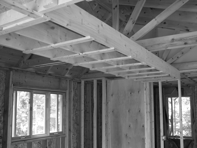
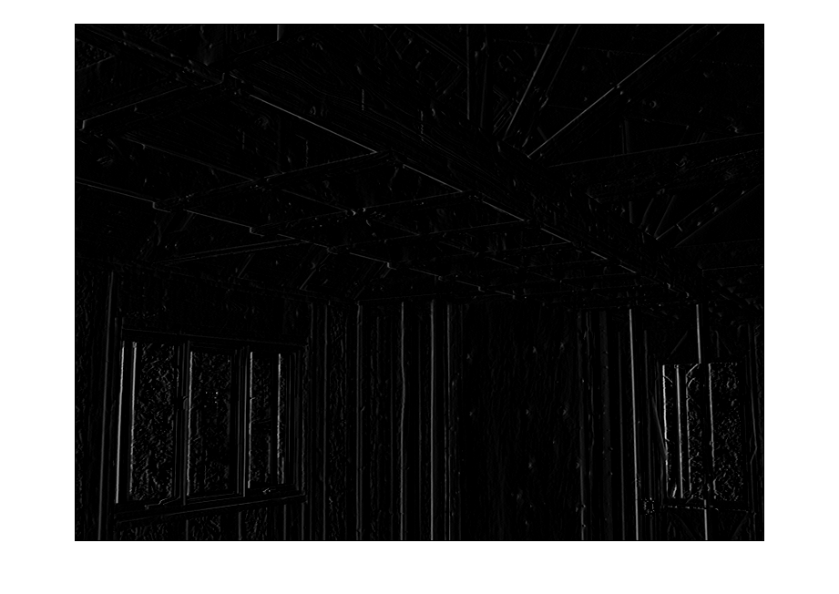
Here we have an gray scale image with a lot of edges. Let’s move our filter into 2 d, but we’ll limit it to enhanceing only the vertical edges by using this pattern:

0	0	0
-1	0	1
0	0	0

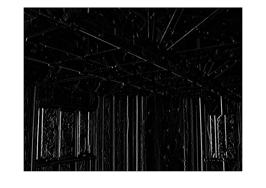
We will modify and use the ApplyFilter Matlab function (code provided at the end) on this image with this filter:

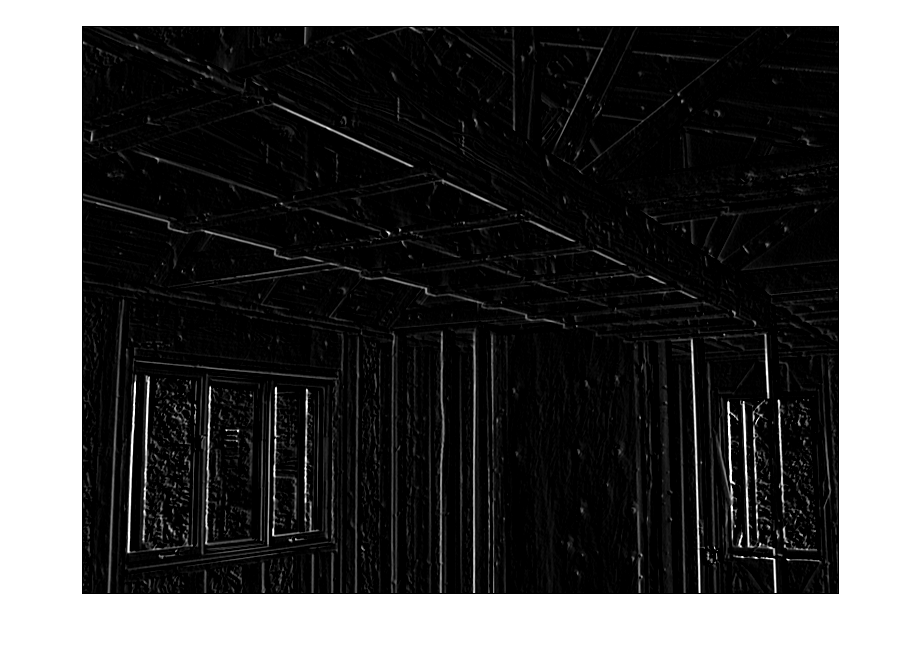
Above we have the image with the vertical lines enhanced. Now we’ll try to pick up some diagonals that point from bottom right to top left. To do that we’ll add another set of coefficients, along the diagonal perpendicular to the lines we want to enhance:

0	0	1
-1	0	1
-1	0	0

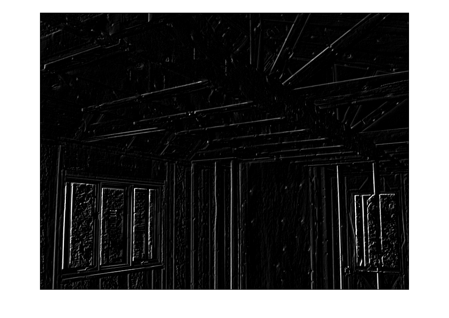
Here we can see the additional diagonal lines picked up. Let’s pull out the other diagonals:

-1	0	0
-1	0	1
0	0	1

 

OK, lastly we’ll pick up all the edges with the full set of coefficients.

-1	0	1
-1	0	1
-1	0	1

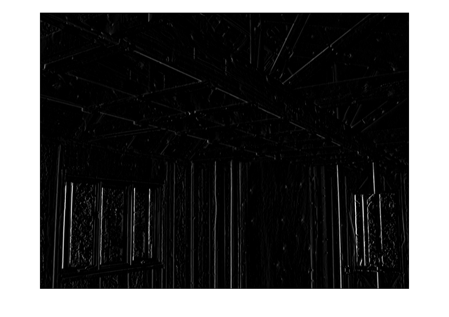
We can see the lines, but, they seem a bit bright. We can put our divide by 2 back in now that we have a “real” image and bring the relative brightness of the lines back into proportion:

This is a more accurate, but perhaps less useful image. We could just as well skip the divide by two if we want the lines to stand out more.

So, that’s all for Part 1!

In Part 2 I’ll discuss  2^nd derivative kernels, and also how to get the angles of the enhanced lines.

Rick Frank

Dominion Software, Inc.

Matlab code:

function [ RESULT ] = FirstDifference( inputVector )

%FirstDifference Demonstrate taking the centered first difference of the input vector, as

%a 1D example of an image processing edge enhancement.

kernel = [-1 0 1];

[rows cols] = size(V);

RESULT = zeros(1,cols);

% loop through the data, but we must focus on 1 pixel inside

% at both ends.

for i = 2:cols-1

temp = 0;

% loop over the “Kernel”, K, which simulates a centered first difference

for j = -1:1

data = inputVector(i+j);

mult = kernel(j + 2);

temp = temp + (data * mult);

end

RESULT(i) = temp;

end

end

function [ RESULT ] = ApplyFilter( inputImage )

%ApplyFilter apply a 3 by 3 filter to the input image

% Modify this kernel as desired.

kernel = [-1 0 1; -1 0 1; -1 0 1]

dbImage = im2double(inputImage);

[rows cols] = size(dbImage);

RESULT = zeros(rows,cols);

% loop through the data, but we must focus on 1 pixel inside

% at both ends.

for aRow = 2 : rows – 1

for aCol = 2 : cols – 1

temp = 0.0;

% loop over the “Kernel”

for rowOffset = -1 : 1

for colOffset = -1 : 1

imageRow = aRow + rowOffset;

imageCol = aCol + colOffset;

data = dbImage(imageRow,imageCol);

mult = kernel(rowOffset + 2,colOffset + 2);

% divide by two if we wish

temp = temp + ((data * mult) * 0.5);

end

end

RESULT(aRow,aCol) = temp;

end

end

end